Faculty of Medicine and Health Sciences
Department of Circulation and medical imaging
Faculty of Medicine and Health Sciences
Department of Circulation and medical imaging
by
Asbjørn Støylen, Professor, Dr. Med
asbjorn.stoylen@ntnu.no
![]()
Deals with the basic physiological concepts; contractility and load, and the relation of deformation parameters to these, diastolic function, event timing and relation to valve function and intraventricular flow and pressures. Any imaging method deals with myocyte shortening, myocyte shortening is always a function of tension versus load, and thus any imaging method and measure is load dependent.
There are two methods for ultrasound deformation imaging, tissue Doppler and speckle tracking. Both methods have advantages and disadvantages, which are dealt with in the ultrasound chapters, but the basic physiology is method independent, so the basic physiology in this chapter is valid for both methods.
This section deals with the basic physiology as seen with various echo methods, and replaces most of
In the physiological aspects, as these were largely overlapping anyway.
There will be discussions of validity on composite measures, these will be based almost solely on physiological principles.
Of course the opposite caveat is also true. Biological plausibility is not evidence of effect, it's at bes hypothesis generating.
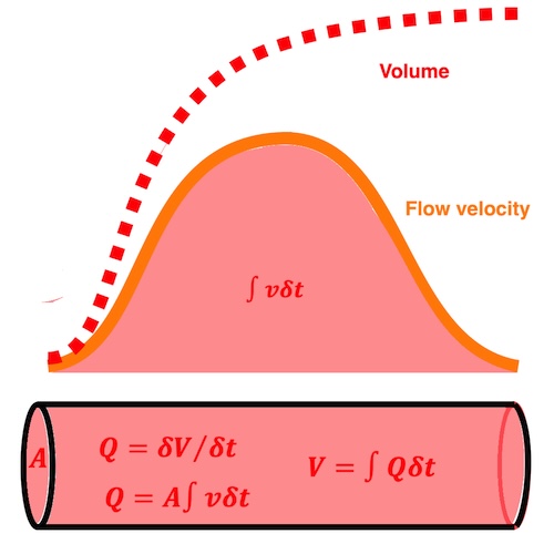
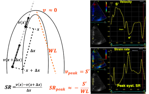
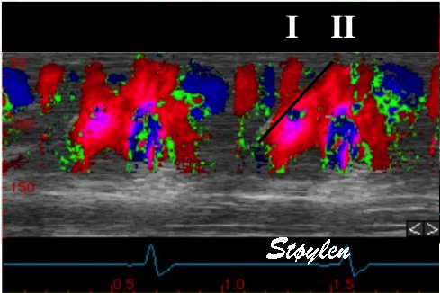
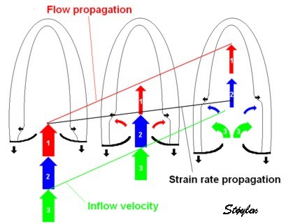
The first temporal derivatives of these parameters are
The spatial derivative of flow is
This is
Systolic deformation is the result of fibre shortening, although in a complex manner.
|
|
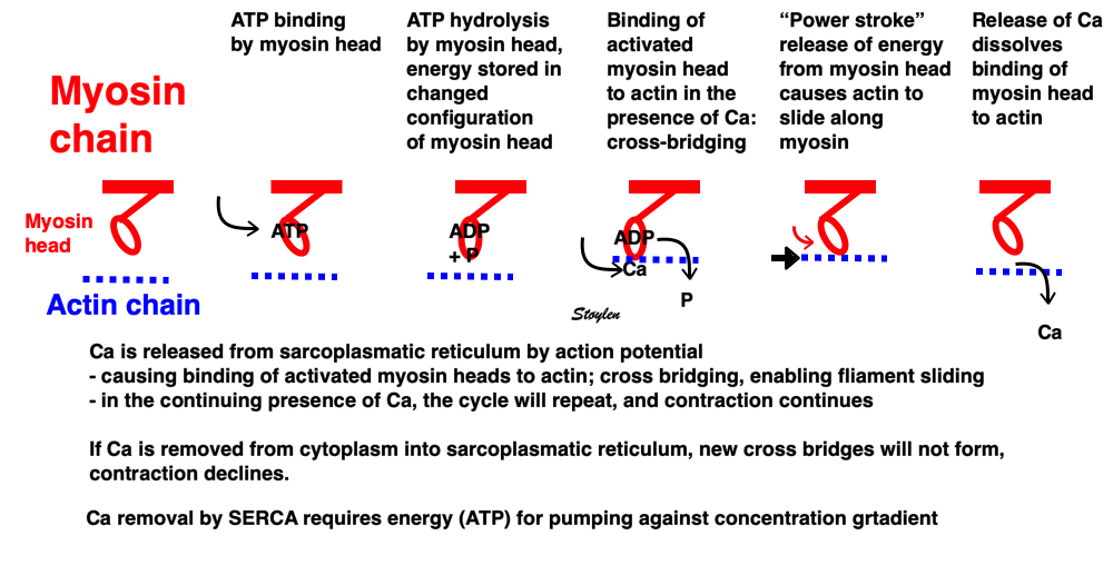
Image of beating isolated myocyte, prepared so the cell fluoresces with the presence of free calcium in the cytoplasm, the cell is stimulated to generate action potential. In systole the cell can be seen to increase free calcium and simultanously shorten. In the cellular diastole, the cell can be seen to elongate, and simultaneously free calcium disappears from the cytoplasm. The isolated myocyte is the completely unloaded situation, where myocyte tension results directly in shortening, and where shortening is a direct measure of contraction.. Image courtesy of Ph.D. Tomas Stølen, cardiac exercise research group (CERG), Dept. of Circulation and Medical Imaging, Norwegian University of Science and technology. | Excitation-tension diagram. The Action potential triggers the influx of calcium, which triggers further release of Ca2+from sarcoplasmatic reticulum. Calcium binds to troponin, and allows activated (by ATP) myosin heads to bind to troponin sites on actin (cross bridge forming) and release energy, causing the filaments to slide along each other, as long as there is a high calcium concentration in the cytoplasm. As the cell membrane repolarised, this triggers the removal of calcium from the cytoplasm, mainly by the SERCA pumping it into the sarcoplasmatic reticulum again. The removal of free calcium is an energy (ATP) demanding, active transport of calcium into the sarcoplasmatic reticulum by SERCA.Thus, obviusly, both contraction and relaxation are ATP demanding processes, and energy depletion will affect both. |
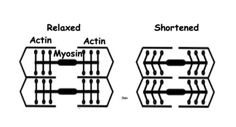
Fibre shortening is not the same as contraction. We have both isometric and isotonic contraction:

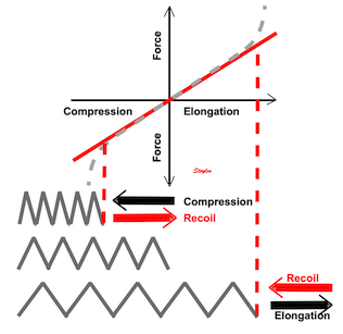
Diagram of mucle sarcomere shortening. Shortening is the result of tension versus load. If the load is higher than the maximal tension the muscle can develop, the muscle will not shorten at all. Actin is still moved along the myosin , but the energy is stored as deformation within the sarcomere without shortening aof the sarcomere. This means that the force generated by contraction is stored as elastic tension in the muscle, and the contraction is isometric The middle figure, retaining the length of the baseline - left). If the load is less than the maximal tension, the muscle will start to shorten when tension equals load, and from there the contraction is isotonic - shortening at constant load. The right sarcomere is shorter than the baseline.
In physiology and pathophysiology, the main object in characterising increased or decreased muscle function is the contractility, which is the ability to develop tension independent of load. As imaging only measures length, the tension must be inferred from knowledge of load. Shortening is the result of tension vs. load as discussed later.
As the muscle uses some time to develop full tension, in most situations there will be a period before tension reaches load (an isometric phase) before tension equals load and the muscle starts to shorten (isotonically) (78).
The concept of load is important for understanding the contractility. Contractility is defined as the inherent capacity of the myocardium to contract independently of changes in the preload or afterload (79).
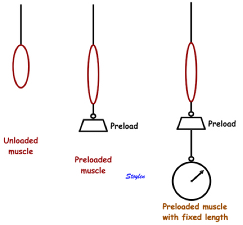
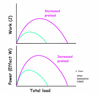
The preload is defined as the load present before contraction starts (79). This is illustrated below left.
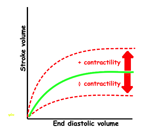
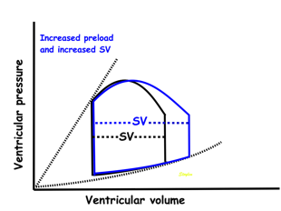
Frank-Starlings law of the heart states: Dilatation is caused when increased venous return or decreased ejection increases end-diastolic volume. This form of dilatation, within physiological limits, increases the heart’s ability to do work. The stroke volume of the heart increases in response to an increase in the the end diastolic volume, when all other factors remain constant. (83)
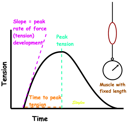
Preload is the force acting on the muscle before contraction starts. Thus, it will stretch the muscle, and induce an increase in muscle tension. This is best explained in isometric experiments, where an isolated muscle is fixed in both ends , and tension is measured by a tensiometer.
|
|
Isometric experiment. Isolated muscle with fixed length, tension measured by a tensiometer. The three measures of tension are the peak rate of force (tension) development, time to peak tension and peak tension. They are all measures of contractile function. | Adding a weight to the muscle without stimulating contraction, will stretch the muscle, before fixating the muscle and adding a tensiometer. This can be achieved without the weight, of course, simply by fixing the muscle at different lengths (pre stretch). |
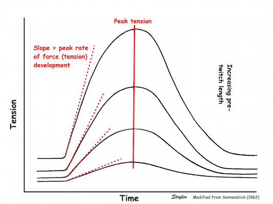
With increasing length by pre stretch, the stretch will both increase passive tension (elasticity), but also increase the active tension developed when stimulated (78).
|
|
Stretching the muscle before stimulation, increases tension. The increase in passive tension will be present at rest, before twitch. During twitch, there is an increase in total tension with increasing pre twitch length. The increase in contractile tension is then the difference between the passive and the total curve. | Isometric twitces with increasing pre-twitch length. In can be seen that as opposed to inotropy, time to peak tension do not increase, even though peak tension does, and, as a consequence of this the rate of force development (as the rise to higher peak during the same time gives higher rate). |
|
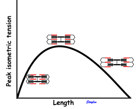
|
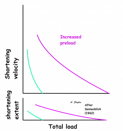
Hypothetical length tension diagram, based on the sarcomere hypothesis, that by increased fibre length initially will increase the overlap between the myosin head regions and the troponin regions on actin, optimising the number of cross bridges that can be formed, and thus the peak tension obtainable. In this model there is an optimal length, then the available number of cross bridges, and thus the peak tension decline again. | Both shortening and shortening velocity can be seen to increase with increasing preload. |
Afterload is force added to the preload as resistance to the muscle shortening. Total load is preload + afterload. This is the force the muscle must overcome ( e. the tension the muscle must develop) in order to shorten, also termed wall stress. This can be expressed as wall stress, the force acting on the wall. This is proportional to both the intracavitary pressure, and radius. Wall stress, however is the tension per cross sectional thickness of the wall, i.e. if the same load is applied to different wall thicknesses, the thickest wall has lowest wall stress per mm thickness.
This is summed up in Laplaces law: Wall stress () is proportional to pressure (P) x radius (r), and inversely proportional to the wall thickness (h):
![]()
In an afterloaded contraction, the muscle must first build up force corresponding to the total load, before it can start shortening. When the force equals the load, further contraction is translated into shortening without tension increase (isotonic contraction). Thus, neither peak force nor time to peak force are relevant measures of contractility.
|
|
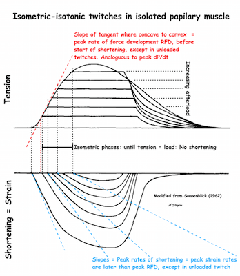
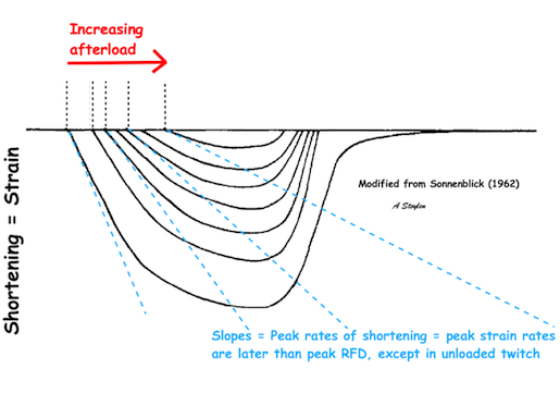
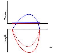
The difference between pre- and afterload is illustrated here. After preload is added, a support is placed, preventing further stretch of the muscle when another weight is added. This second weight is the afterload. When the muscle contracts, it has to develop a tension that is equal to the total load, before it can shorten. If the peak force is higher than the total load, the muscle will then shorten without generating more tension, in an isotoniccontraction. | Isotonic isometric twitches tension diagrams above, length diagrams below. From the diagrams, it is evident that shortening only starts after tension have reached load, and then, the tension is constant while the muscle shortens. Thus the first part of an unloaded contraction is also shortening, while the first part of a loaded contraction is isometric, becoming isotonic after tension equals load. Peak rate of force generation (RFD), occurs during the isometric phase (except in the unloaded phase, where there is no tension development). Peak rate on the other hand occurs during the first part of the shortening, after tension = load, and is thus later than peak RFD. The figure also shows that shortening decreases as load increases, as more of the total work is taken up in tension development. This experiment shows that both peak rate of shortening and peak shortening, i.e. peak strain rate are affected by afterload. Both peak shortening and peak rate of shortening are affected by pre- and afterload.The curves are explained further below. |
|
|
|
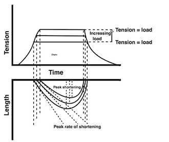
Length tension diagram of a muscle twitch in an isolated muscle preparation. The muscle takes some time to develop the tension that equals the load, and during that period the contraction is isometric, with no shortening. Shortening starts when tension equals load. When the muscle relaxes, relaxation induces shortening until tension again equals load, after that relaxation is isometric. | Series of twitches with different loads. All twitches follow the same tension curve, i.e. shows the same contractility, but as load increases, shortening starts at later time points, and the shortening time as well as the extent and rate of shortening decrease. | Series of twitches with the same load, but with different contractility (ability to develop tension). With decreasing contractility, it takes longer to develop tension = load, the period of shortening as well as the extent and rate of shortening decrease. |
Looking at the whole heart cycle, there is a complex interaction between tension increase and devolution, and shortening and elongation whioch is discussed here.
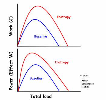
Contractility is defined as the inherent capacity of the myocardium to contract independently of changes in the preload or afterload (79). The contractility decreases in myocardial failure and with betablocker, but increases with inotropic stimulation, such as adrenaline, noradrenaline or calcium.
|
|
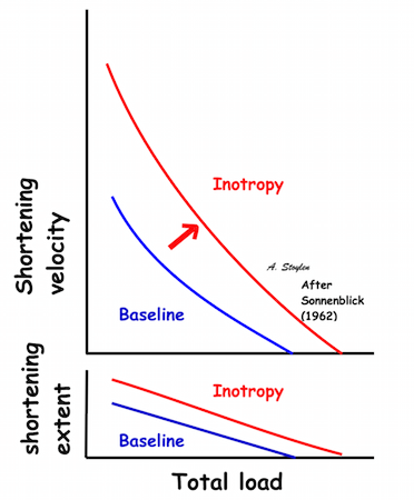
Shortening velocity and total shortening, Relation to preload and total load. Both shortening and velocity can be seen to decrease with increasing afterload (total load), but increase with preload. | Shortening velocity and total shortening, Relation to total load and inotropy. Both can be seen to increase with inotropy, but decrease with load. |
As we see, both increased preload and inotropy wil increase the muscles ability to develop tension, and thus the shortening and shortening velocity in an isotonic experiment. This can also be shown alternatively:
|
|
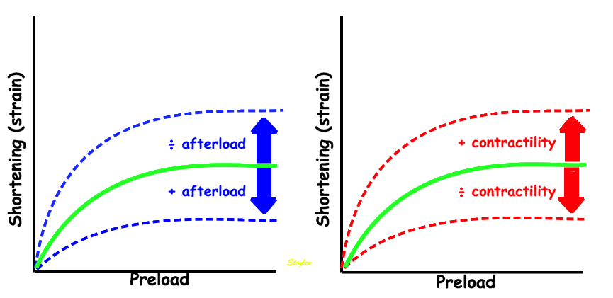
Stretching the muscle before stimulation, increases tension. The increase in passive tension will be present at rest, before twitch, and is equal in baseline and inotropic state. During twitch, there is an increase in total tension with increasing pre twitch length. The increase in contractile tension is then the difference between the passive and the total curve. At a certain length, active tension starts to decline, even if passive and total tension still increases. This effect is additional to the effect of inotropy. | Myocardial shortening vs pre-, afterload and contractility. shortening increases with preload, as shown in both panels, although to a certain extent, until the preload insensitive zone (where active tension starts to decline, but passive tension still increases). Shortening is the resultant of force vs. afterload, the higher the afterload, the less the shortening, for a given contractility. Contractility is the load independent part of force development. The higher the contractility, the more the shortening for a given afterload. |
Thus, both shortening (strain) and peak rate of shortening (peak strain rate) is load dependent, and not independent measures of contractility, and looking at imaging, it is difficult to discern between reduced contractility and reduced load as shown below. This means, of course, that both strain and strain rate are load dependent.
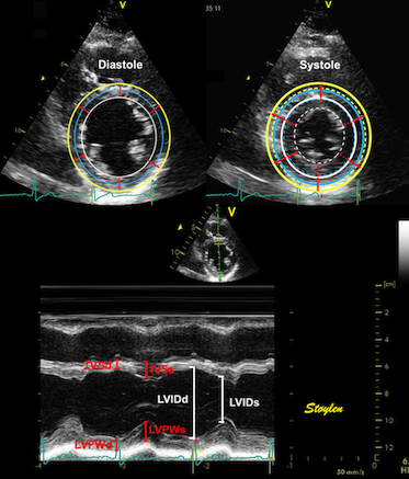
Cardiac volumes
|
|
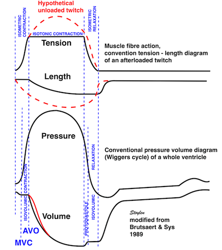
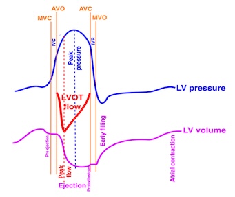
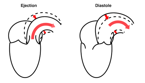
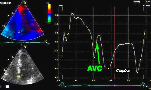
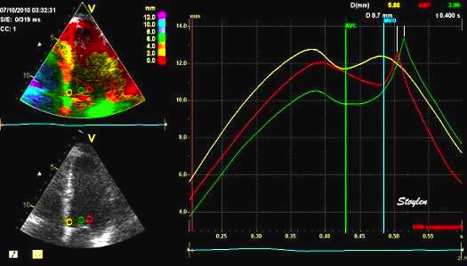
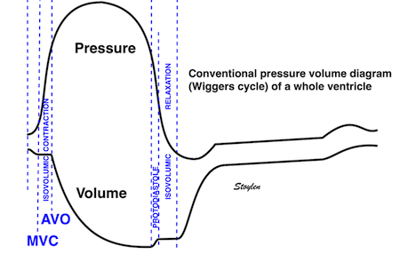
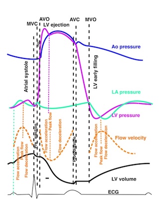
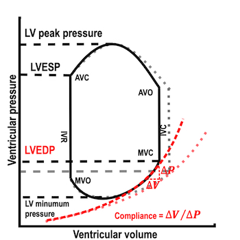
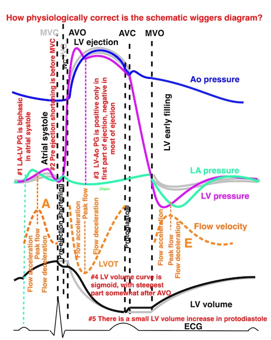
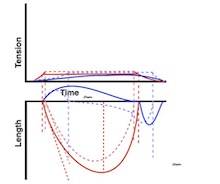
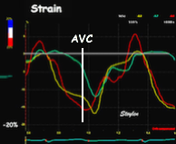
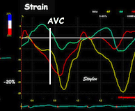
Isotonic isometric twitches tension diagrams above, length diagrams below. From the diagrams, it is evident that shortening only starts after tension equals load, and thenthe muscle shortens isotonically. Peak rate of shortening (peak strain rate) is at the start of shortening, and then declines (the slope of the shortening curve) . Only in the totally unloaded situation does the muscle start to shorten art start contraction. In the loaded situations, peak rate of force generation (RFD), occurs during the isometric phase, before peak rate of shortening. Peak shortening (peak strain), on the other hand, is at the end of the isotonic phase. | Comparing a tension length diagram of an isotonic/isometric twitch, and a pressure/volume (Wiggers)diagram. I've added the division of pre ejection into protosystole and IVC as discused above. The ejection period is not isotonic, as pressure increases and then decreases, and the myocardial tension must follow a similar course. Thus the tension increase is only during the first part of ejection, and then tension decline, so last part of ejection is relaxation. However, the volume curve will reflect the fibre lengthening and shortening, which makes is very obvious that strain and strain rate are about volume changes. Peak shortening is at en ejection, when volume is smallest. The conventional Wiggers diagram as shown by Brutsaert (black) describe the steepest volume decrease at the time of AVO, but as flow takes some time to accelerate, the peak volume decrease rate (which equals peak flow rate, must be slightly delayed after AVO). This is shown by the red part of volume curve. |
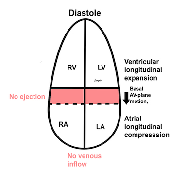
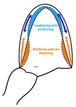
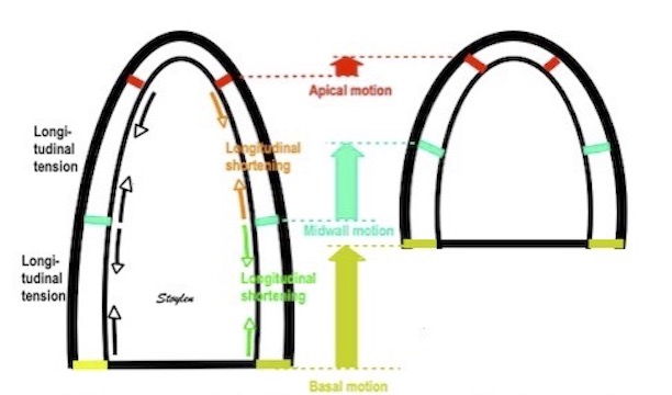
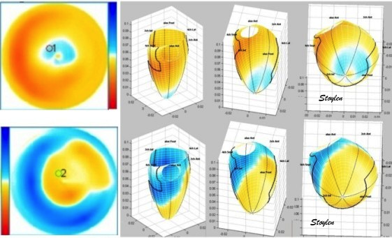
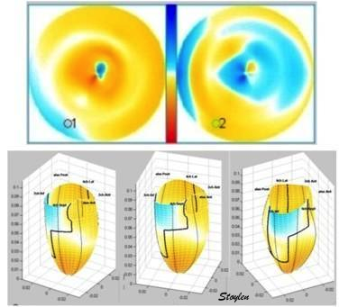
Volume changes and muscle fibre length changes are analogous, of course, as systolic decrease in volume has to be accompanied by muscle shortening, diastolic increase in volume by muscle lengthening. As described in the basic concepts page, there is systolic circumferential and longitudinal shortening, and fibre shortening, while transmural strain is not fibre shortening, but thickening.
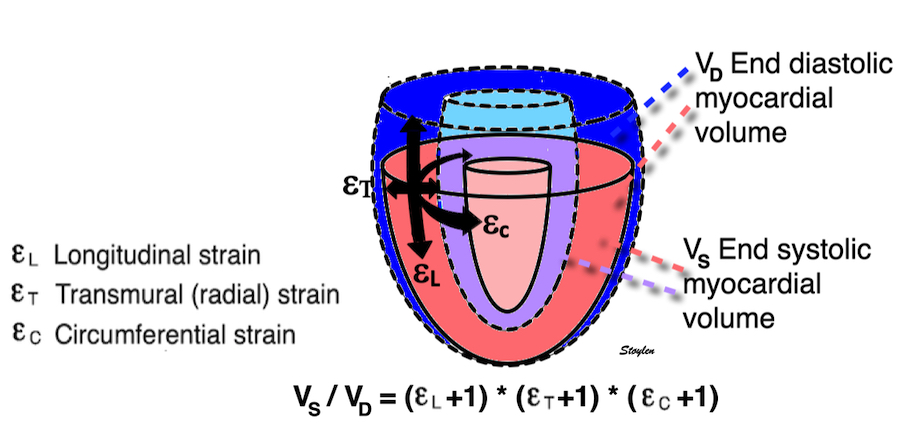
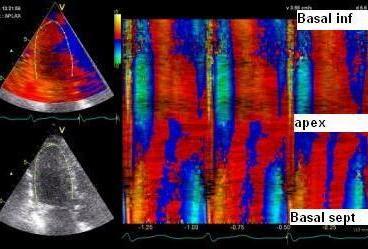
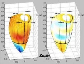
Deformation of the myocardium. In systole, there is volume reduction, as well as longitudinal and circumferential shortening. The strains are related to volume change, as shown above.
However, the strains are coordinates of the myocardial deformation, not direct measures of fibre shortening. While circumferential shortening is geometry related, longitudinal shortening is the one that is most closely related to volume change, and thus to fibre shortening.
|
|
|
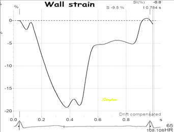
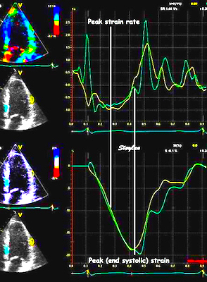
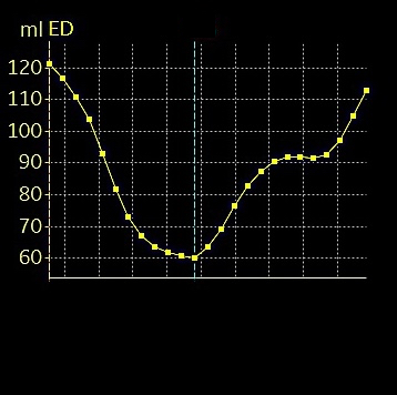
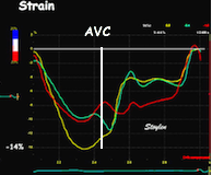
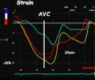
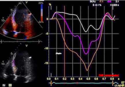
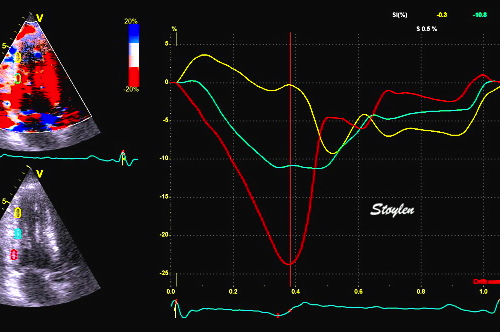
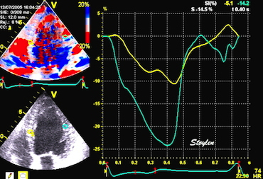
Shortening curves related to afterload, modified from the figure above. The shortening in percent, is equivalent to the longitudinal strain of the muscle. | Strain curve from a normal subject. The strain curve is fairly similar to the shortening curves to the left. | The picture shows a detailed LV volume curve from a healthy person by MUGA scintigraphy, showing how analoguous the strain curve is to the volume curve. |
So now, we can relate the physiological findings in isolated muscle to the volume changes originally descrtibed in Frank Starlings law:
|
|
Acute increases in end diastolic filling, will increase the stroke volume along the curve shown. This effect was observed with both increased venous pressure, but also with decreased stroke volume in previous beat, resulting in an increased EDV. Within physiological limits there is an increase, but with increasing dilatation, there will be less response. However, at least in normal hearts, there is little evidence for a descending limb of the curves. It is important that Frank Starlings law is about acute volume changes, not chronic changes as in hypertrophy or dilation. The curve shows the preload (which is | SV versus afterload. Shortening is the resultant of force vs. afterload, the higher the afterload, the less the SV, for all preloads. |
Thus, global strain rate and strain are not load independent, as explained above. One would almost say of course. Force is the primary effect of contraction. Deformation is secondary to force, and depends on load. Motion is the summation of deformation. The systolic volume change of the ventricle is related to the resistance, which again is a function of both pressure and vascular resistance. What we measure with deformation parameters, is only the changes in volume, and thus the wall deformations.
thus, physiologically the rate and amount of longitudinal shortening should decrease with increasing load. Anything else would be counter intuitive.
The heart cycle can basically be described in terms of volume changes, which in turn are the function of ejection and filling:
This is slightly simplified, as will be explained later.
The true isovolumic contraction time (IVC) is defined from MVC to the start of ejection. Thus, in this phase there is no volume change, and, hence, no deformation.
This phase it on the other hand, the period of most rapid pressure rise, peak dP/dt, which occurs during IVC, close to the AVC (105). This represents the most rapid rate of force development (RFD). As this phase is basically not influenced by aortic pressure, it is largely afterload independent, except for the Laplac e effect: It's important to realise that the Frank-Starling balance and the pressure volume loop both relate to acute changes in ventricular volume. The physiologic differences in EDV between individuals, and in chronic LV enlargement, are not responsible for preload. On the other hand, by the law of Laplace:
![]()
LVEDV is part of the afterload, the tension must be proportional to the radius: As the intraventricular pressure acts on a larger surface, and thus the force that has to be generated must be proportional to the surface area for the same pressure. dP/dt increases with inotropy (106, 107)
On the other hand, dP/dt is preload dependent as any contraction measure (106, 107).
|
|
Muscle twitches, showing that the most rapid rise of tension occurs during isometric contraction, but the highest rate of shortening occurs in the bunloaded muscle before peak RFD. | Peak rate of pressure rise, which is the closes correlate to the rate of force/tension development. This occurs during IVC |
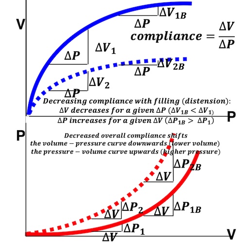
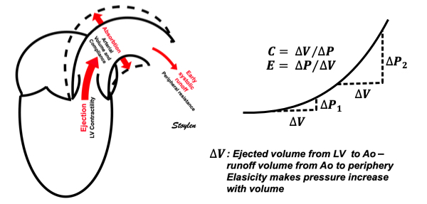
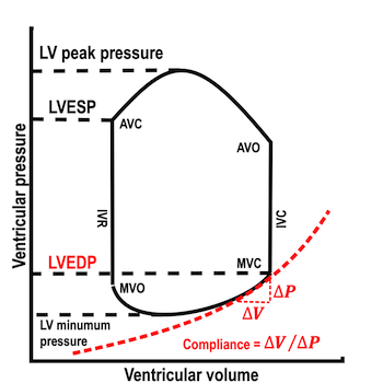
Compliance (distensibility) is defined as C = ![]() V /
V / ![]() P, i.e. how much does the volume increase for a given increment in pressure. Elastance is the inverse value E =
P, i.e. how much does the volume increase for a given increment in pressure. Elastance is the inverse value E = ![]() P /
P / ![]() V, i.e. how much does the pressure increase for a given increment in volume.
V, i.e. how much does the pressure increase for a given increment in volume.
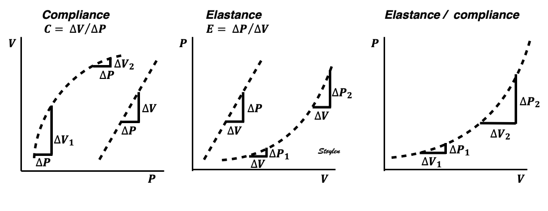
Compliance describes the volume a a function of pressure, and hence, should ideally be described in a volume-pressure diagram. The figure shows linear compliance, as well as decreasing compliance (decreasing volume per pressure increment), as can be seen in an elastic system. | Elastance, despite simply being the inverse of compliance, describes pressure as a function of the volume, and thus is best describel in a pressure-volume diagram. Here is shown linear elastance, as well asincreasing pressure for the same volume increments, as can be seen in an elastic system. | The pressure volume volum loops is generally described in a pressure volume diagram, i.e. showing volume as ordinate and pressure as abscissa. However, both compliance and elastance can be shown in this diagram, obviously, as both describe the ratios between pressure and volume increments. |
The length - tension relation in isolated muscle is equivalent to the pressure - volume relation in the intact heart. To go into the concept of cardiac work and contractility, the whole heart cycle has to be considered. Basically, pressure-volume loops are useful concepts for visualising and explaining the relations between stroke volume, pressure, contractility and LV work.

The pressure-volume loop on the right is derived from the pressure and volume curves on the left. It is basically a tool to assess and explain the relations between contractility, load and output. Isovolumic contraction (IVC) is between MVC and AVO, there being no volume change, this is a true isometric contraction. Isovolumic relaxation is between AVC and MVO, this is the isometric phase of relaxation. Pressure volume diagram of a heart where pressure is plotted against volume, a pressure-Volume loop (PV-loop). Pressure-volume loops are useful concepts for visualising and explaining the relations between stroke volume, pressure, contractility and LV work.The version shows the cardiac phases, with the same simplifications as the Wigger's diagram to the left; rapid filling is shown as a passive event, and as valve openings and closures are shown at pressure crossover. Time runs around the loop in a counterclockwise direction. The width of the loop is equal to the stroke volume. The top of the diagram shows the pressure curve during ejection, and the height of the loop is the systolic - diastolic pressure difference. The tangent to the end systolic pressure-volume, is the ventricular elastance ![]() P /
P / ![]() V.
V.
In filling of any hollow organ, the elastance is usually taken to mean how much pressure increase a given volume increment generates as described above, and the definition of elastance is ![]() P /
P / ![]() V.
V.
End systolic LV elastance is defined as the slope of the straight line trough the end systolic pressure volume corner of the pressure volume loop. It has been shown to be nearly linear trough multiple pressure volume loops obtained by manipulating the pre and afterload. However, the straight line has not been shown to be crossing the zero point, i.e. the volume is not necessary zero when pressure is zero.
End systolic elastance is a function of LV emptying. Thus this must be taken to mean how much pressure the LV must generate for a given volume ejection (SV), but the definition is ![]() P /
P / ![]() V, and thus conforms with the definition of elastance.
V, and thus conforms with the definition of elastance.
The PV loop shows the relation between load, SV and contractility in acute changes.
|
|
|
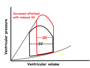
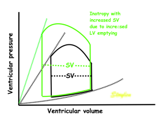
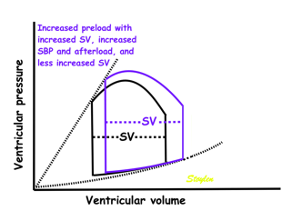
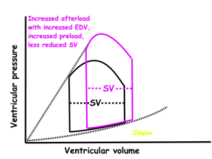
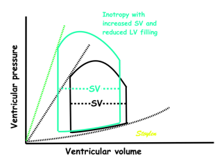
Effect of preload. Increased preload (increased LVEDV - the right side of the curve moves right, the loop becomes wider), will, through the Frank-Starling balance increase stroke volume. This increased stroke volume will be ejected at the same pressure, thus returning to the same point on the ESPVR line. | Effect of afterload. Increased afterload (increased SBP moving the top of the curve upwards), will reduce the stroke volume. The end systolic point moves up the ESPVR line, shortening the width of the loop, i.e reduced SV. | Effect of inotropy. Inotropy shifts the ESPVR line to the left, thus increasing the force and LV emptying, increasing stroke volume through reduced LVESV, but also increasing the pressure, both through increased contractile force and increased volume being ejected into the vascular bed. |
|
|
|
In reality, an increased SV will cause increase in SBP, causing an increased afterload on the same beat, thus reducing the effect on SV somewhat, through interaction between pre- and afterload. | In reality, an acute increase in afterload, will reduce emptying (increased LVEDV), so on the next beat, the preload is increased, partly offsetting the effect of afterload on SV. | In reality, decreased LVESV, without increased venous return, will in the next beat result in reduced LVEDV, thus offsetting the effect of inotropy somewhat by reduced preload. |
Ventricular elastance, is thus a load independent measure of contractile force (84).
In reality, this index is not easily obtainable in the clinic, even in continuous invasive monitoring, as volume measurements are not available in routine monitoring. But in animal experiments, using conductance catheters, where multiple pre- and afterload manipulations can be done, and where the ESPVR can be obtained by linear regression, it serves as a reference method, to test other contractility indices.
However, the LV elastance may not be a perfect gold standard anyway.
- Firstly, using end ejection for end systole, means that measurements are done at a point in time where the myocardium is in relaxation (but not relaxed) phase as discussed below.
Several studies have found that the ESPVR is not a straight line, curvilinear depending on contractility (85, 86), and afterload (87, 88).
Peak systolic pressure volume relation might be closer to the real thing, but is not easily discernible.
- Secondly, as we'll see later, the true end systolic volume is not easily defined due to the protodiastolic volume decrease as discussed below.
Finally, however, of course these volume considerations are only related to acute changes. In inter individual differences in healthy individuals, as well as in LV dilation, the EDV is not a measure of preload, and the PV-loops can only be interpreted in relation to the individual. PCWP, on the other hand, is a measure of preload, that is relatively standardised and thus a more universal measure of preload when applied across individuals, although it does not take the Laplace effect into consideration, the LV volume will stioll contribute to after- (or total load).
Volume: It's important to realise that the Frank-Starling balance and the pressure volume loop both relate to acute changes in ventricular volume. The physiologic differences in EDV between individuals, and in chronic LV enlargement, are not responsible for preload. On the other hand, by the law of Laplace:
![]()
LVEDV is part of the afterload, the tension must be proportional to the radius: As the intraventricular pressure acts on a larger surface, and thus the force that has to be generated must be proportional to the surface area for the same pressure.
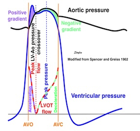
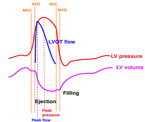
Pressure: The pressure, is the systolic pressure, which varies during the ejection:
| |
The ejection period is not isotonic, as pressure increases and then decreases, and the myocardial tension must follow a similar course. Thus the tension increase is only during the first part of ejection, and then tension decline so last part of ejection is relaxation. The volume curve (as given by Brutsaert - black) is erroneous. Due to the acceleration of blood, the peak flow rate, and thus the rate of volume decrease must be somewhat later than the AVO, as shown by the red curve. | With conventional pressure/flow recordings, the peak pressure / tension is around mid ejection, but looking at flow, peak flow through aortic ostium is much earlier during ejection. As flow rate equals the rate of volume decrease, peak flow must indicate peak rate of volume decrease. |
2. The tension increase is closely related to distension of the large vessels. The elasticity (compliance) of the arterial (especially the aortic) wall. During ejection, the volume ejected into the aorta and distends it. The more distensible the aortic wall (the higher the compliance ![]() V /
V / ![]() P - the volume increase per pressure unit), the less the pressure in the aorta will rise, and the lower the CAP. The stiffer the aorta, the less it will be distended (the less the compliance) for a given pressure increase, or conversely the more the pressure has to be increased in order to inject a certain volume (stroke volume) into the aorta. Thus, increased arterial stiffness will increase the systolic pressure, and hence, the afterload (108).
P - the volume increase per pressure unit), the less the pressure in the aorta will rise, and the lower the CAP. The stiffer the aorta, the less it will be distended (the less the compliance) for a given pressure increase, or conversely the more the pressure has to be increased in order to inject a certain volume (stroke volume) into the aorta. Thus, increased arterial stiffness will increase the systolic pressure, and hence, the afterload (108).

During ejection, the volume is ejected into the aorta, which is distended, storing energy in the elastic properties, and then contracting again during diastole, acting as a diastolic pump, with energy stored from systole.
The ventricle ejects the full stroke volume into the arterial bed during systole. However, there is systolic run off to the periphery, so the volume distending the arterial bed is less then the stroke volume. Thus the ![]() V distending the artery is less than the total SV, and the difference is determined by the peripheral resistance, and the pressure drops toward end systole.
V distending the artery is less than the total SV, and the difference is determined by the peripheral resistance, and the pressure drops toward end systole.

Ventricular ejection distends the arterial bed, and the elastic properties results in pressure increase related to the volume, and the compliance decreases as the volume increases. However, the run-off into the arterial bed, during systole, leads to the end systolic volume (and pressure) is less than the total SV. This run off is determined by the peripheral resistance.
The pressure is inversely related to the arterial compliance, or directly related to the elastance ![]() P /
P / ![]() V (the pressure increase per volume unit), and is the inverse of arterial compliance. As the pre arteriolar arteriaø bed is elastic, there is thus no reason to believe that the arterial elastance is linear. Arterial eleastance could also be both end diastolic, peak systolic or end systolic.
V (the pressure increase per volume unit), and is the inverse of arterial compliance. As the pre arteriolar arteriaø bed is elastic, there is thus no reason to believe that the arterial elastance is linear. Arterial eleastance could also be both end diastolic, peak systolic or end systolic.
Thus, what is called "effectve arterial elastance" is defined as SV / ESP. But this, of course defines a straight line slope, even if this is improbable, so this concept is only valid for end systolic pressure and SV. However, using ESP takes into account the whole of the SV, but also the fall i pressure from peak to end systole, which is a function of the run off during systole, and thus peripheral resistance. Thus, it is a measure of afterload taking both components of the arterial bed into account (260 - 262).
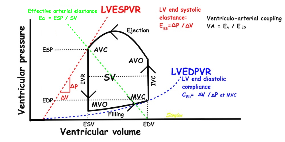
PV-loop illustrating effective arterial elastance. The arterial elastance is a measure of how much pressure the stroke volume generates in the arterial bed,
and is simply EA = ESP/SV, which is the slope of the line crossing zero at the end diastolic volume, and the point defined by the end systolic volume and pressure. It is the arterial pressure increase in relation to the stroke volume. The ventricular elastance is LV end systolic elastance, the pressure generated by the ventricle fpr ejecting the stroke volume; EES = ESP/ESV. But then, given that the theoretical volume of the LV for pressure P =0 is V = 0, then EA / EES = (ESP/SV)/(ESP/ESV) = ESV/SV = (EDV - SV)/SV = EDV/SV - 1 = 1/EF - 1. Thi9s of course is not necessarily the case, but depends on the placement and slop of the LVESPR line. Thus the concept of VA coupling simply eliminates the pressure, and ends up with a load dependent measure of LV performance as a result of this load!

Pulse wave reflection at the level of the aortic root. In the upper panel, pulse wave propagation velocity is lower, and the reflected wave from the previous heartbeat arrives after AVC, and will then augment the diastolic pressure only, not contributing to afterload. In the lower panel, due to a higher PWP, the reflected wave arrives before the AVC, and will augment the systolic pressure, which willl be higher than the peripheral pressure. Systolic pressure augmentation will thus add to the afterload.
Finally, of course, the body regulates both the cardiac performance and load in relation to the needs of the body:
Thus, of course, all factors of cardiac performance in the intact body may change in relation to the body's needs. But this may be a very complex regulation of the contractile state (by variations in inotropy), preload (by variations in venous return - venoconstriction; giving load dependent increase in contraction) and afterload by varying arterial tone (which again is often balanced by inotropy). The final variable is the cardiac output.
This means that heart rate is in itself a determinant for especially shortening rate, and more indirectly, shortening, and secondly to stroke work and cardiac output.
The HUNT3 (16) and 4 (249) are two of the largest normal single center studies of Echocardiography in the world. Both are similar in size (HUNT3 1266 vs HUNT4 1412), and with normal age distribution.
HUNT 3 | HUNT 4 | |||
Women | Men | Women | Men | |
Number | 673 | 623 | 788 | 624 |
Age (years) | 47.8 (13.6) | 50.6 (13.7) | 57.2 (12.4) | 57.8 12.4) |
BMI (Kg/m2) | 25.8 (4.1) | 26.5 (3.4) | 25 (4) | 26 (3) |
BP (mmHg) | 127 / 71 (17/10) | 133 / 77 (14/10) | 127 / 72 (18/9) | 131 / 78 (17/10) |
There was a slight difference in mean age. As many of the measurements are age related, the age distribution is important in comparing populations.
HUNT 3 was acquired in 2006 - 2008, HUNT 4 in 2017 - 2019. Thus the echo populations are two different cohorts, although there was some overlap, as participants from HUNT3 were invited to participate in HUNT4, but the individuals paticipating in both were aged 20 years, and the comparison will give further data an ageing.
Both normal studies excluded patients with heart disease, diabetes and hypertension.
HUNT3 was taken on GE Vivid 7, and analysed in EchoPAC version BT06, (except strain and strain rate, which was analysed in the proprietary segmental strain analysis software.
HUNT4 was acquired on GE Vivid E95 and analysed on EchoPAC version 203. Thus there were technical developmental differences as well.
The two studies differ in much of the measurement methodology, meaning that comparison is interesting from a methodological viewpoint, but also in looking at age and sex relations across methods. In linear dimension measurements, HUNT 3 used mainly M-mode, HUNT4 B-mode.
Dimensions of the ventricle is closely related to the functional measures. While the motion indices of displacement and velocity are dimension unrelated, strain and strain rate are relative deformation measures, and thus related to dimensions. Thus changes in dimensions will relate to changes in strain and strain rate. The HUNT study, being ta large study of normals has published normal values, related to age and gender (19):
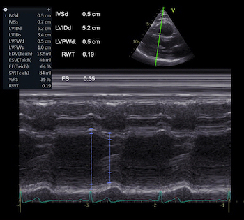
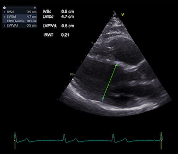
Conventional left ventricular cross sectional measures from M-mode in the HUNT3 study by age and gender, raw and indexed for BSA. SD in parentheses.
Age (years) | N | IVSd | IVSd/BSA | LVIDd | LVIDD/BSA | FS (%) | LVPWd | LVPWd/BSA | RWT | RWT/BSA |
Women | ||||||||||
<40 | 207 | 7.5 (1.2) | 4.2 (0.6) | 49.3 (4.2) | 27.5 (2.6) | 36.6 (6.1) | 7.7 (1.4) | 4.3 (0.6) | 0.31 (0.05) | 0.17 (0.03) |
40–60 | 336 | 8.1 (1.3) | 4.5 (0.7) | 48.8 (4.5) | 27.3 (2.8) | 36.5 (6.9) | 8.3 (1.3) | 4.6 (0.7) | 0.33 (0.05 | 0.19 (0.03) |
> 60 | 118 | 8.9 (1.4) | 5.1 (0.8) | 47.8 (4.8) | 27.4 (3.1) | 36.0 (9.1) | 8.7 (1.4) | 5.1 (0.8) | 0.37 (0.07) | 0.22 (0.04) |
All | 661 | 8.1 (1.4) | 4.5 (0.8) | 48.8 (4.5) | 27.4 (2.8) | 36.4 (7.1) | 8.2 (1.4) | 4.6 (0.8) | 0.34 (0.06) | 0.19 (0.04) |
Men | ||||||||||
<40 | 128 | 8.8 (1.2) | 4.3 (0.6) | 53.5 (4.9) | 26.1 (2.6) | 35.5 (6.9) | 9.2 (1.3) | 4.5 (0.7) | 0.34 (0.06) | 0.17 (0.03) |
40–60 | 327 | 9.5 (1.4) | 4.6 (0.7) | 53.0 (5.5) | 26.0 (3.0) | 35.8 (7.4) | 9.7 (1.4) | 4.7 (0.7) | 0.37 (0.07) | 0.18 (0.03) |
> 60 | 150 | 10.1 (1.6) | 5.1 (0.9) | 52.1 (6.4) | 26.3 (2.9) | 36.0 (8.0) | 10.0 (1.3) | 5.1 (0.7) | 0.39 (0.07) | 0.20 (0.04) |
All | 605 | 9.5* (1.5) | 4.6† (0.8) | 52.9* (5.6) | 26.0† (2.9) | 35.8 (7.5) | 9.6* (1.4) | 4.7† (0.7) | 0.37 (0.07) | 0.18 (0.04) |
Total | 1266 | 8.7‡ (1.6) | 4.6 (0.8) | 50.8‡ (5.4) | 26.7 (2.9) | 36.1 (7.3) | 8.9 (1.6) | 4.7 (0.7) | 0.35 (0.07) | 0.18 (0.04) |
*p<0.001 compared to women. †p<0.01 compared to women. ‡Overall p<0.001 (ANOVA) for differences between age groups. RWT: relative wall thickness.
Wall thicknesses and LVIDD correlated with BSA (R from 0.41 - 0.48), Thus, all values were consistently higher in men due to this. FS, of course, did not correlate with BSA, and was thus gender independent. Wall thicknesses increased with age (R=0.33), and LVIDD decreased with age, as opposed to older studies (34, 35), possibly because of their smaller size.
FS remained constant between age groups, in accordance with other studies.
The values are M-mode derived.
In HUNT3, the upper normal cut off for RWT would be 0.49, which is relevan for M-mode derived values.
Relative wall thickness is generally considered to be a body size independent measure, as both wall thicknesses and LVIDD are body size dependent, the RWT, supposedly, is normalised for heart size, and hence, for body size. Interenstingly, in the HUNT study this was not the case, although correlation with BSA was very modest (R=0.18). This probably do not warrant normalising RWT for BSA. More pronounced was correlation with age (R=0.34), increasing from 0.31 to 0.37 in women, and from 0.34 to 0.39 in men. For M-mode derived values this means that the cut off for RWT would be 0.51 in the upper age groups, for both sexes.
The age dependency is a logical consequence of the unchanged LVIDd and increasing wall thickness, and has been shown also previously (33).
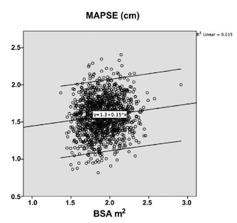
Relation of RWT and BSA in HUNT3. This shows that RWT is not perfectly aligned with body size. | RWT and age in HUNT3. This shows a more marked dependence of RWT and age, so age related normal values is probably warranted. |
Comparing with the values from HUNT4 (249), which were measured in 2D the values according to aghe and sex can be found in the original publication.:
Age (years) | IVSd (mm) | LVIDd (mm) | LVIDs (mm) | FS (%) | LVPWd (mm) | RWT |
Women | ||||||
20 - 39 | 6.8 (1.2) | 49 (4) | 33.3 (4.0) | 0.32 | 6.6 (0.9) | 0.27 |
40 - 59 | 7.4 (1.3) | 48 (4) | 33.0 (3.7) | 0.31 | 6.9 (1.0) | 0.30 |
60 - 79 | 8.1 (1.5) | 45 (4) | 30.9 (4.2) | 0.31 | 7.5 (1.1) | 0.35 |
> 79 | 8.2 (1.0) | 41 (4) | 28.1 (3.0) | 0.31 | 7.7 (1.2) | 0.39 |
All | 7.7 | 47 | 32 | 0.32 | 7.2 | 0.32 |
Men | ||||||
20 - 39 | 7.9 (1.3) | 52 (4) | 35.2 (4.3) | 0.32 | 7.3 (1.0) | 0.29 |
40 - 59 | 8.7 (1.3) | 52 (5) | 35.9 (4.5) | 0.31 | 8.0 (1.2) | 0.32 |
60 - 79 | 9.2 (1.5) | 50 (5) | 33.9 (4.8) | 0.32 | 8.3 (1.2) | 0.35 |
> 79 | 9.3 (1.7) | 48 (6) | 34.6 (3.9) | 0.28 | 8.2 (0.8) | 0.36 |
All | 8.9 | 51 | 34.9 | 0.32 | 8.1 | 0.33 |
Total | 8.2 | 49 | 33.3 | 0.31 | 7.6 | 0.33 |
Values are taken from (249). All age differences were significant) Values were corrected for the numbers in each age class before averaging by me. FS and RWT are calculated by me from the basic measurements, and likewise corrected for numbers.
What we see is that the M-mode derived values of HUNT3, are slightly higher than the 2D derived values from HUNT 4, for wall thickness and chamber diameter. The sex and age distribution of the subjects are about the same in both studies, although the age related decline in LVIDd is steeper in HUNT4.
The NORRE study (250), however, had intermediate values; IVSd 8.6 mm and LVPWd 8.8 mm, although closer to HUNT3. LVIDd was fairly close in HUNT 3 and 4, somewhar smaller in NORRE (44.3 mm), age related values for linear dimensions are not given. Mean FS in NORRE can be calculated to 33%.
Thus, the NORRE study seems to confirm the bias between M-mode and 2D derived measures, being lower than HUNT3.
This consistent with a statistical bias towards skewed measures in M-mode, which tend to be corrected in 2D (224), so values in HUNT3 may be valid for M-mode measures, but will overestimate the true values, and is not transferable to 2D derived measures.
|
|
|
Reconstructed M-mode with a fairly straight cross angle between the M-mode line and the LV long axis. | Reconstructed M-mode from the same loop, but with the M-mode line crossing the LV long axis at a skewed angle, showing thicker walls and wider cavity, due to the angulation. | B-mode measurement across the ventricle in the same loop. Wall thicknesses are similar to the straight angle M-mode. LVIDd (and hence, RWT) are slightly different as the measurement line does not cross the posterior wall at exactly the same point. |
However, the relation between values, and relations with age, seems to be valid across the methods. Decreasing LVIDd but increasing WT with increasing age was found in both HUNT3 and 4, so these relations are not method specific. FS do not seem to differ very much between age groups in either study. Theoretically, skewed measurements would not affect the ratio of the measured values (RWT and FS). However, as we see, both RWT and FS are slightly lower in HUNT4, and in the NORRE study the mean FS was 0.33 as well. Skewed measures should not give increased ratios per se, but, angulation will also be affected by the AV plane motion, so there are more systematic errors than just angulation.
The cut off for RWT in HUNT 4 would be ca 0.47 over all. Mean RWT in the NORRE study can be calculated to 0.39, higher than both HUNT 3 and 4, confirming that the cut off seems to be to low. While RWT increases with age in both studies. As RWT is derived from wall thicknesses which increases significant with age (249) and LVIDd which decreases significant with increasing age, (249), the increase in RWT has to be significant as well.
Increasing wall thickness and LVIDd with higher BSA, and relative wall thickness thus also have to increase with increasing age as diameter decreases and wall thickness increases in both studies. The cut off for RWT in HUNT 4 would be ca 0.47 over all, and increasing by age, possibly around 0.50 for the upper age groups, still higher than previous normal cut off values (224).
The age relation is not taken into account in current guidelines, but as upper normal limit increases by age, age related values should be warranted.
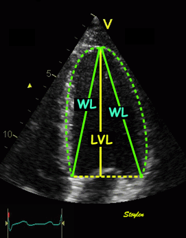
Left ventricular length and external diameter is also important in an evaluation of the total strain images. In the HUNT3 study, we initially measured wall length, from the mitral annulus to the apex, which will over estimate the LVL, but is proportional (19). Later, we refined this to an ellipsoid model, allowing to calculate the mid cavity LV length (65) as shown below.
|
|
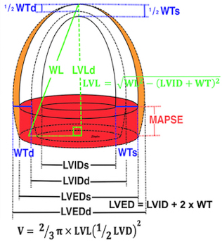
Left ventricular length. Wall lengths were measured in a straight line (WL) in all six walls from the apex to the mitral ring. This wil underestimate true wall lengths (dotted, curved lines), but will be more reproducible, as the curvature may be somewhat arbitrary. LVL was calculated as mean of all four walls, thus overestmating true LVL (yellow line) slightly, but again the arbitrary placement in the middle of the ostium will result in lower reproducibility, while taking the mean of six measurements will increase it. | Ellipsoid model of the left ventricle. All basic measures are linear, and the ellipsoid model assumes symmetrical wall thickness, declining to half in the apex, mitral annular diameter constant; equal to ventricular end systolic diameter, as LV diameter decreased by 12.8% is systole while the fibrous mitral annulus may be assumed to be more constant. LVL is calculated by the pythagorean theorem, using 1/2 LVIDd plus 1/2 WTd. |
Left ventricular external diameter, is simply the sum of the wall thicknesses and LVIDd. From the geometric calculation, we found LV internal and external lengts (assuming apical wall thickness in both systole and diastole to be 50% of basal wall thickness:
Left ventricular wall length and external diameter by age and gender from the HUNT3 study, raw and indexed for BSA..
Age (years) | N | LVEDD (cm) | LVEDD/BSA (mm/m2) | LWVL (cm) | LWVL/BSA (cm/m2) | LVWL/LVEDD | LVELd (mm) | LVILd (mm) |
Women | ||||||||
<40 | 207 | 6.45 (0.48) | 35.9 (2.7) | 9.4 (1.6) | 5.23 (1.00) | 1.46 (0.26) | 91.0 (6.2) | 87.2 (6.1) |
40–60 | 336 | 6.52 (0.52) | 36.5 (3.2) | 9.1 (1,7) | 5.08 (0.95) | 1.40 (0.27) | 88.5 (6.0) | 84.3 (5.9) |
> 60 | 118 | 6.52 (0.52) | 37.7 (3.5) | 8.9 (1.3) | 5.08 (0.79) | 1.36 (0.23) | 85.0 (5.9) | 80.1 (5.9) |
All | 661 | 6.51 (0.51) | 36.5 (3.2) | 9.1 (1.6) | 5.13 (0.93) | 1.41 (0.27) | 88.7 (6.4) | 84.6 (6.4) |
Men | ||||||||
<40 | 128 | 7.16 (0.53) | 35.0 (2.9) | 10.3 (1.7) | 5.02 (0.88) | 1.44 (0.25) | 99.6 (6.4) | 95.0 (6.4) |
40–60 | 327 | 7.22 (0.58) | 35.0 (3.2) | 10.0 (1.8) | 4.84 (0.89) | 1.39 (0.26) | 97.3 (7.4) | 92.5 (7.4) |
> 60 | 150 | 7.22 (0.68) | 36.5 (3.1) | 9.5 (1.8) | 4.80 (0.97) | 4.80 (0.97) | 92.1 (7.8) | 87.1 (7.8) |
All | 605 | 7.21 (0.59) | 35.3 (3.1) | 9.9 (1.4) | 4.86 (0.91) | 1.38 (0.27) | 96.5 (7.8) | 91.7 (7.8) |
Total | 1266 | 6.84 (0.65) | 36.0 (3.2) | 9.5 (1.8) | 5.00 (0.93) | 1.40 (0.27) | 92.4 (8.1) | 88.0 (7.9) |
SD in perentheses, LVELd: Diastolic external length LVILd diastolic internal length. p < 0.001.
It is logical that LVEDd increased both with BSA (R=0.60) and modestly with age (R=0.11, the unchanged LVIDd being part of it, dilutes the effect of wall thickness) (19).
Left ventricular length, on the other hand, increased with BSA (R=0.29), but decreased with age (R = -0.12).
Left ventricular external diameter, is calculated from the published values as the sum of the wall thicknesses and LVIDd. Values were corrected for the numbers in each age class by me.
Values from HUNT4 , measured in 2D the values according to age and sex can be found in the original publication (249).: LV lengths were exported from the volumetry tracings in 2D (Dalen H personal communication), meaning they represent inner length.
Age (years) | IVSd (mm) | LVIDd (mm) | LVPWd (mm) | LVEDd (mm) | LVILd-4ch (cm) | LVILd2ch (cm) |
Women | ||||||
20 - 39 | 6.8 (1.2) | 49 (4) | 6.6 (0.9) | 62.4 | 8.5 (0.6) | 8.6 (0.8) |
40 - 59 | 7.4 (1.3) | 48 (4) | 6.9 (1.0) | 62.3 | 8.3 (0.6) | 8.4 (0.6) |
60 - 79 | 8.1 (1.5) | 45 (4) | 7.5 (1.1) | 60.6 | 7.9 (0.6) | 7.9 (0.6) |
> 79 | 8.2 (1.0) | 41 (4) | 7.7 (1.2) | 56.9 | 7.1 (0.5) | 7.3 (0.5) |
All | 7.7 | 47 | 7.2 | 61.5 | 8.1 | 8.2 |
Men | ||||||
20 - 39 | 7.9 (1.3) | 52 (4) | 7.3 (1.0) | 67.2 | 9.7 (0.6) | 9.7 (0.6) |
40 - 59 | 8.7 (1.3) | 52 (5) | 8.0 (1.2) | 68.4 | 9.2 (0.6) | 9.4 (0.7) |
60 - 79 | 9.2 (1.5) | 50 (5) | 8.3 (1.2) | 67.5 | 8.9 (0.6) | 8.9 (0.6) |
> 79 | 9.3 (1.7) | 48 (6) | 8.2 (0.8) | 65.5 | 8.5 (0.5) | 8.4 (0.5) |
All | 8.9 | 51 | 8.1 | 68.0 | 9.1 | 9.2 |
Total | 8.2 | 49 | 7.6 | 64.3 | 8.5 | 8.6 |
Values are taken from (249). All age differences were significant, although not tested for LVEDD. As in HUNT3, we se that the age effect on LVEDd is diluted, by the decreasing LVIDd and increasing WT.
In HUNT3, the mean left ventricular internal length was calculated from wall lengths to 88 mm. In HUNT4, the internal LV length was 85 mm.
Disregarding the separate age group > 80, which has no comparable group in HUNT3 (and which are small), we see that internal length decline from 87 - 80 mm in women and 95 - 87 in men, while in HUNT 4 the lengths declined from 85 - 79 mm in women and 97 - 89 in men.
Thus both studies confirm a decline in both internal diameter and length with increasing age.
Fundamental findings are summarised below:
Fundamental findings in the HUNT study: With increasing BSA, both wall thickness, internal diameter (and hence, external diameter) and relative wall thickness increase, showing that neither measure is independent of body size (or heart size). The length / external diameter, however, remains body size independent, being a true size independent measure. Differences are exaggerated for illustration purposes. | With increasing age, both wall thickness (and hence, external diameter) increase, while internal diameter is age independent. Left ventricular length decreases, and hence length / external diameter decreases, and i a measure of age dependent LV remodeling. This has implication for LV mass calculation. Dimension changes are exggerated for illustration puposes. |
The ratio L/D did not correlate with BSA in HUNT3, was near gender independent (although the difference was significant due to the high numbers), but declined somewhat more steeply with age (R = -0.17). In HUNT4, the ratio between external diameter and internal length was 1.32 in women and 1.34 in men, but declined with age.
This has some important corollaries:
Applying the linear measures to an elliptical model of the left ventrcle, allowed the estimation of LV volumes (471).
Ellipsoid model of the left ventricle. All basic measures are linear, and the ellipsoid model assumes symmetrical wall thickness, declining to half in the apex, mitral annular diameter constant; equal to ventricular end systolic diameter, as LV diameter decreased by 12.8% is systole while the fibrous mitral annulus may be assumed to be more constant.
The ellipsoid model has some limitations. Being symmetric, it do not conform totally to the shape of the LV, which is assymmetric, as in other model studies.
An indication of this was that while all linear measurements were near normally distributed, there was a greater skewness in the calculated volunes:
Comparing skewnesses of the distributions of the linear measures (which is small), with the calculated volumes (which is significantly (greater), seems to indicate a systematic error in the volume data from the model.
Despite this, findings were interesting.
Age | LVEDV(ml) | SV(ml) | EF(%) | Myocardial volume d (ml) |
Women | ||||
<40 | 111.6(21.6) | 76.3(16.4) | 68(6) | 87.0 (19) |
40-60 | 106.9(21.7) | 72.7(17.0) | 68(6) | 92.8 (19.6) |
>60 | 97.9(19.7) | 65.4(16.9) | 66(9) | 95.6 (18.9) |
Total | 106.8(21.8) | 72.6(17.3) | 68(6) | 91.4 (19.6) |
Men | ||||
<40 | 144.8(30.5) | 96.1(22.9) | 66(8) | 125.3 (23.6) |
40-60 | 138.1(31.1) | 92.2(23.8) | 67(8) | 129.7 (25.3) |
>60 | 126.3(33.7) | 84.1(25.7) | 66(8) | 128.2 (26.8) |
Total | 136.6(32.2) | 91.0(24.4) | 67(8) | 128.4 (25.3) |
All | 121.1(31.1) | 81.4(22.9) | 67(8) | 101.4 (27.9) |
LV volumes in HUNT4
Volumes in HUNT 4 are 2D measurement derived, values given are taken from (249).
Comparing with the values from HUNT4 (249), which were measured in 2D, the values according to age and sex can be found in the original publication.:
Age (years) | LVEDV(ml) | SV(ml) | EF(%) |
Women | |||
20 - 39 | 114 (26) | 68 | 60 |
40 - 59 | 102 (19) | 62 | 61 |
60 - 79 | 84 (19) | 51 | 60 |
> 79 | 67 (7) | 41 | 62 |
All | 94 | 57 | 61 |
Men | |||
20 - 39 | 145 (28) | 84 | 58 |
40 - 59 | 136 (29) | 81 | 60 |
60 - 79 | 119 (27) | 71 | 60 |
> 79 | 104 (18) | 62 | 59 |
All | 128 | 76 | 59 |
Total | 109 | 66 | 60 |
SV is calculated from EDV and ESV, corrected for the numbers in each age class before averaging.
Compared to the ellipsoid model from M-mode derived values, LVEDV is lower, but the relation to age, with declining values in increasing age are the same. This of course follows from the simultaneous age dependent decrease in both LVIDd and LVILd by age in both studies. Myocardial volume is not calculated in HUNT4.
The NORRE study shows even lower EDV, but LVEDV decrease with age too.
As we have already shown, left ventricular wall thickness increased with age, LV diameter was unchanged, while LV wall length decreased (19). However, LV volume increased by age (65), this effect being more profound in women.
Myocardial volumes were not calculated in HUNT4. The NORRE study gives increasing myocardial mass (which in practice is only myocardial volume × 1.05) in women, with mean 146 g in men and 112 g in women.
But tThe HUNT 3 population despite exclusion of patients with history or treatment for hypertension, had an increasing mean SBP and DBP with increasing age, due to an increasing number with BP above hypertensive levels:
A: Mean BP showing an age related increase, above 60 about half is in the hypertensive level >140/90. B: LV volume in the different BP groups (results were not different if 140/90 was used). There is significant higher volumes in the >130/80 group, but in neither group was there any significant increase with increasing age.
There was a weak, but significant correlation of LV volume with age (R=0.14, p<0.001), but neither in linear regression nor partial coorrelation was there any significant increase with age, indicating that the age effect is mainly an BP effect.
Myocardial compressibility in relation to strains is discussed in the fundamental concepts section.
The volume ratio by strains is
![]()
Given myocardial incompressibility,
![]() ,
,
if the myocardium is compressed during systole,
![]() .
.
In the HUNT3 study, using the strain product on linear measures, the strain product, being equal to the volume ratio was 1.009 (1.0136 - 0.99851) using straight line wall measures (longitudinal strain -16.3%), and 0.9957 (1.003 – 0.98896) using mid ventricular line (longitudinal strain -17.1%). However, speckle tracking tends to measure higher GLS, because of the shortening due to inward tracking of the wall thickening, and wall thickening varies too much between studies to give any meaning of the strain product at all. The answer cannot be given by strains. For speckle tracking, we know that the resolution, and hence the tracking is different in the axial and lateral direction, so the values are not necessarily inter related in a proper way,
In the model study, however, myocardial volumes could be estimated. Here, we found a myocardial volume reduction in systole of 3.28 ml, or 2.5% of myocardial volume, 4.8% of SV.
This corresponds to a Vs/Vd of 0.975 (SD 0.112), 95%CI ((0.969-0.981) .
But as the model has limited accuracy, this is not normative either. Our main finding was that this compressibility, however, was not related to age, BP or BSA.
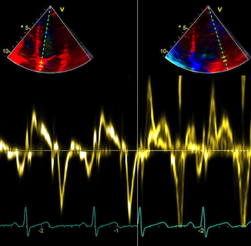
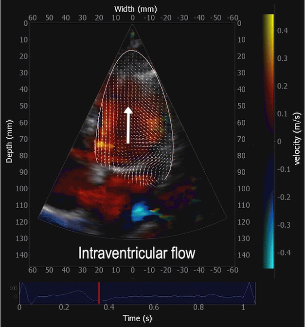
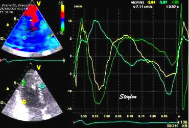
The full heart cycle is composed of the interactions between tissue deformation, flow and pressure in a complex manner. The intraventricular flow is an important part of the total picture.
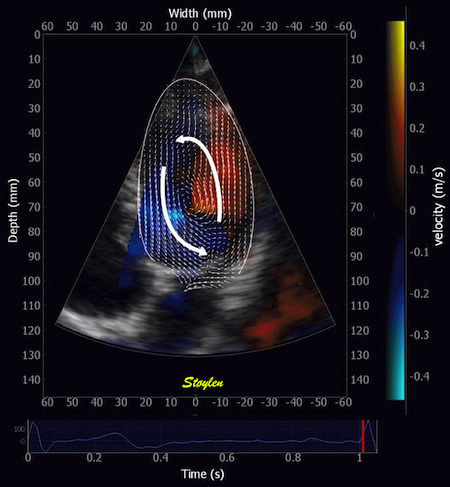
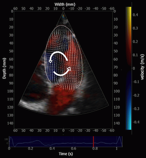
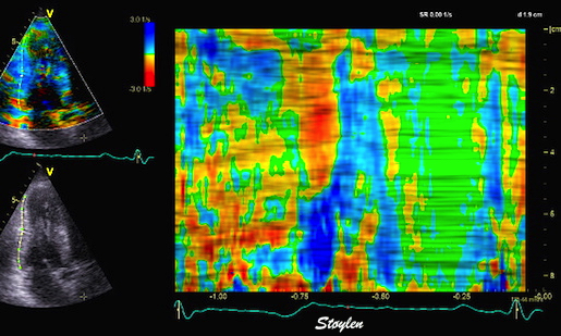
Combined high framerate tissue Doppler and vector flow imaging, showing a vortex in the LV. Image courtesy of Annichen S Daae.
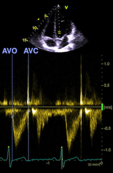
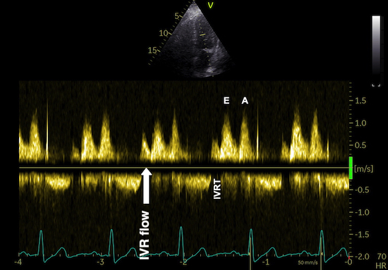
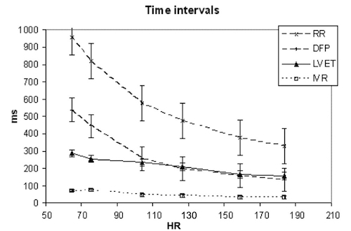
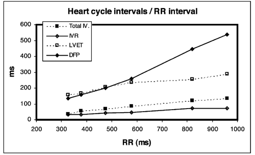
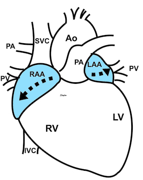
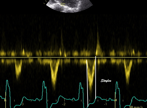
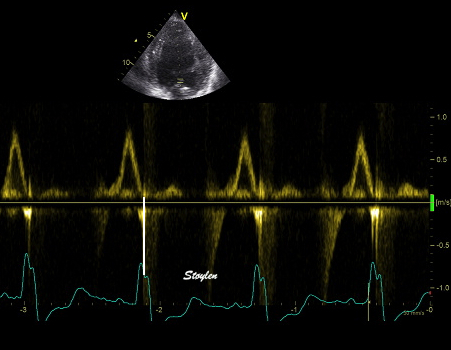
The main intervals of the heart cycle is defined by the valve closures and openings. That means start and end of flow, but with the right positioning of the sample volume /beam, it can also capture the valve closure clicks.
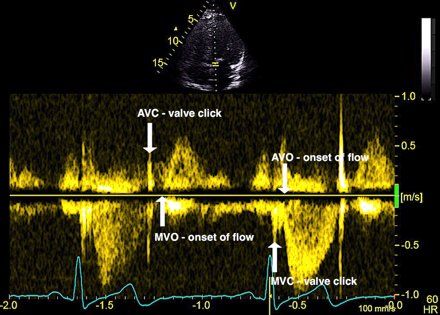
With the right positioning if the sample volume, all left sided valve closures and openings can be registered simultanepously. Valve closures can be seen as clicks, and valve openings can be seen by the start of flow.
Valve opening and closures then can define the main intervals of the heart cycle, IVC, LVET, DFP and IVR.
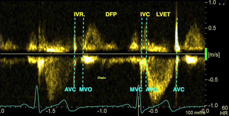
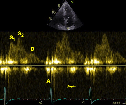
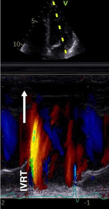
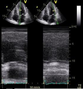
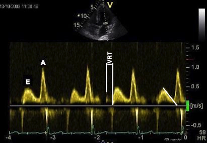
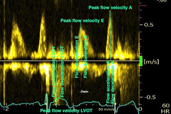
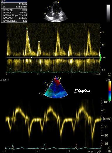
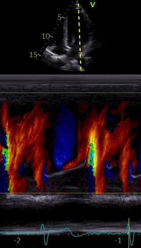
Pulsed wave Doppler with sample volume positioned between the aortic and mitral ostia. Both start and stop of the flows, as well as the valve closure clicks are seen, dividing the heart cycle into the four main phases, ejection, diastolic filling, and between them the isovolumic contraction and relaxation phases..
Tissue Doppler and deformation imaging, howebver have given increased understanding of the basic physiology. Looking at the short phases of the heart cycle, like pre ejection, isovolumic relaxation, and early and late diastole, velocity and strain rate are the most useful, as explained here.
The pre ejection period, is the period from start of ECG, to the AVO (i.e.) the start of ejection (110). It consists of:
The electromechanical activation consists of electrical conduction of the signal from the AV-node through the His' bundle and the anterior and posterior left hemi-bundles. Early experimental and invasive studies seemed to show that there is initial endocardial activation almost simultaneously in mid septum and mid lateral wall, after 0 - 15 ms after onset of ECG (111, 112), but this will be partly concomitant with electromechanical delay at the cellular level. Then, there is electromechanical delay at the cellular level, the action potential generating Calcium influx, again generating release of more calcium form the SR, resulting in onset of cell contraction through actin-myoisin cross bridges. This process takes about 20 - 30 ms (113).
|
|
Excitation-tension diagram. After Cordeiro. The Action potential triggers the influx of calcium, which triggers further release of Ca2+from sarcoplasmatic reticulum. Calcium binds to troponin, and allows activated (by ATP) myosin heads to bind to troponin sites on actin (cross bridge forming) and release energy, causing the filaments to slide along each other, as long as there is a high calcium concentration in the cytoplasm. | Image of beating isolated myocyte. The myocyte is treated with an agent that fluoresces in the presence of free calcium in the cytosol. We see that the cell lightens and shortens simultaneously; stimulation causes an increase in free calcium (released mainly from the sarcoplasmatic reticulum), causing the cell to become lighter. The free calcium is the trigger for the binding of ATP, and the formation of activated cross bridges between actin and myosin, and the subsequent rotation and release, which leads to the buildup of tension in, or shortening of the cell. Image courtesy of Ph.D. Tomas Stølen, cardiac exercise research group (CERG), |
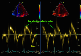
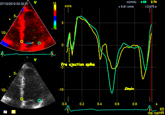
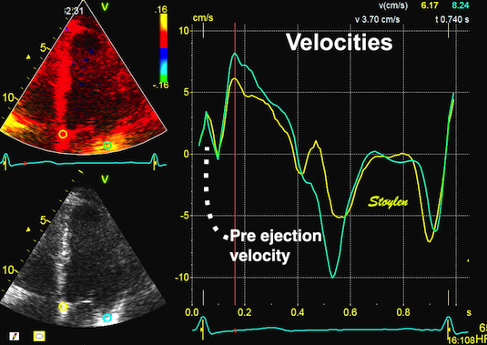
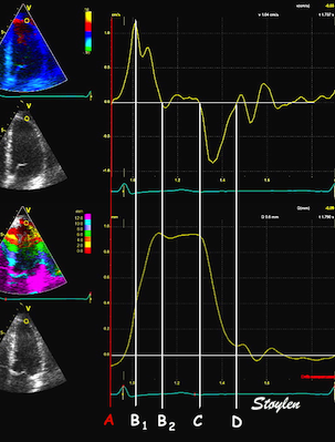
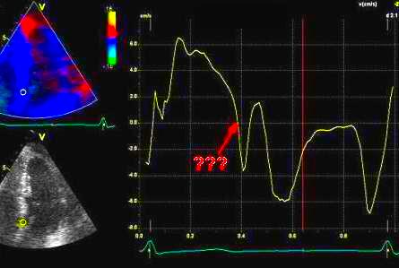
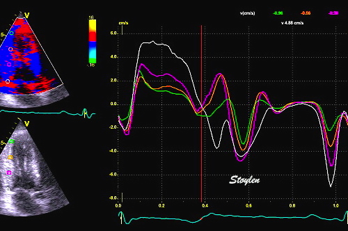
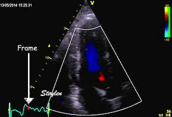
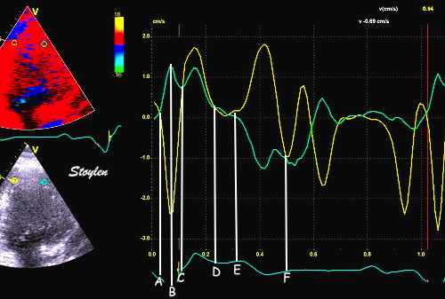
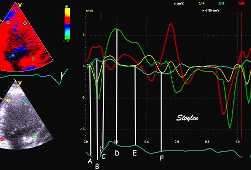
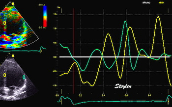
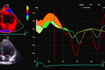
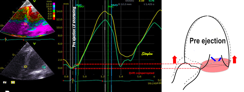
With tissue Doppler, it became evident that before ejection, a short positive velocity spike was visible. It was visible in both septum and the lateral wall (72), and it corresponded to a very small pre ejection apical displacement as seen by M-mode and displacement traces.

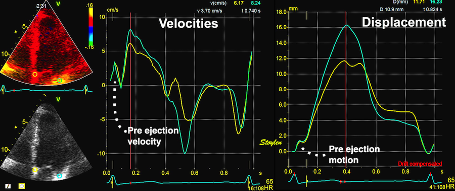
Pre ejection velocity is seen as a small, positive velocity spike before the main motion of the ejection phase, and, correspondingly, a small apiucal motion that can be discerned both in the M.mode and displacement traces. This pre ejectiopn motion is present both in the septum and the lateral wall.
Pre ejection spike can be seen to be lower than peak ejection in most instances | ||
|
|
|
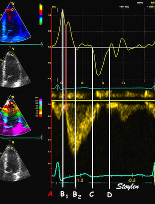
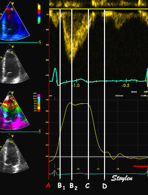
-by spectral tissue Doppler | by colour tissue Doppler | and by speckle tracking. |
The timing of this event has been shown to precede MVC (72).
The pre ejection spike thus occurs BEFORE MVC, as seen here (valve openings and closures from Doppler flow - different cycles). | MVC is concomitant with the stop of pre ejection apical motion. |
It has been suggested to be passive rebound after atrial contraction. This has been suggested, but the pre ejection spike is seen also in atrial fibrillation (114, 117). Rebound after atrial relaxation is present, though, and can be demonstrated, both with and without (as in AV-block) succeeding ventricular contraction, but the timing in relation to the following systole depends on the PQ time. What we see, is that after the a' wave, there may be some rebound oscillations visible in long PQ time or dropped beats, which normally would be dampened by the stiffening of the ventricular myocardium by the onset of contraction.
|
|
|
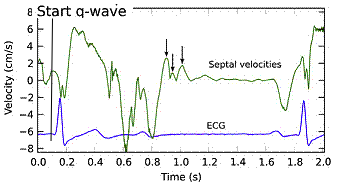
Ultra high frame rate tissue Doppler from the base of the septum a subject with atrial fibrillation. Even with no atrial activity, there is pre ejection velocity spikes, showing them to be ventricular in origin. | Ultra high frame rate tissue Doppler from the base of the septum a subject with 1st degree AV block. (This is a highly trained, healthy subject, the AV block is physiological)Three spikes are seen before ejection (arrows). Here, the initial spike must be atrial recoil, coming before start of the the QRS, it cannot be ventricular i origin. Even the second spike may be atrial, or a fusion of an atrial bounce and ventricular contraction. | Ultra high frame rate tissue Doppler from the base of the septum a subject with 2nd degree AV block, as seen by the second P-wave following the first heartbeat, with no QRS nor ejection velocities. The atrial recoil can be seen as three velocity spikes (arrows), indicating that the mitral ring bounces. However, this is in a situation without LV myocardial tension. At start of the first heart cycle, there may be some fusion between atrial recoil and ventricular contraction as seen by the timing. |
If PQ time is very long, the atrial rebound and pre ejection spikes become separated:
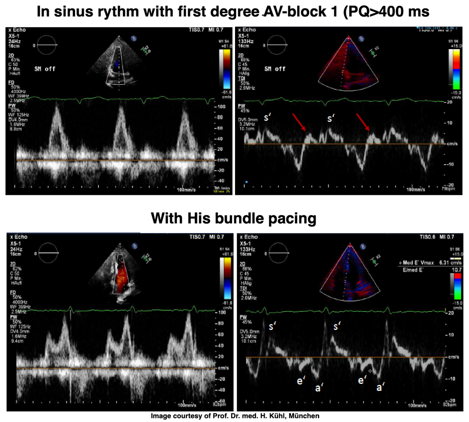
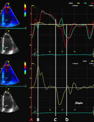
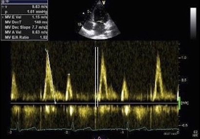
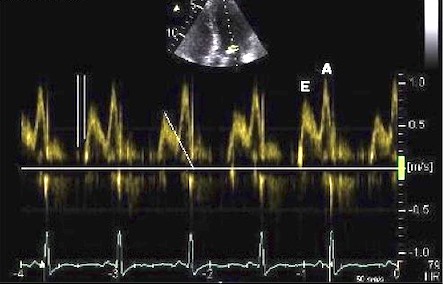
PW Doppler of mitral flow and tissue Doppler from a patient with a PQ time > 400 ms. This pushes the A wave forward to the preceding heartbeat, causing EA fusion as explained elsewhere, but increases the interval between atrial and ventricular systole. After the a' wave in tissure Doppler there is a clear positive wave, that can be seen before the normal pre ejection spike, and may represent a rebound from atrial contraction. With HIS pacing on, the PQ-time is normalised, and both EA fusion and the rebound wave are abolished, the latter may be dampening with the onset of ventricular myocardial contraction (stiffening). The normal pre ejection spike, however, is enhanced. Images courtesy of Prof. Dr. med. H. Kühl, Chefarzt, Klinik für Kardiologie und Internistische Intensivmedizin, Klinikum Harlaching, München.
With ultra high frame rate (1200 FPS) ultrasound, (HFR IQ data), where both MV M-mode and TDI was reconstructed from the same cycle, and the velocity spikes were comp+ared to a reconstructed MV M-mode, MVC was seen to come after the pre ejection spike. In a study of ten healthy subjects, time intervals from start of ECG to start of the initial pre ejection velocity spike in the septum was 22.7 ms, and from this to MVC was 29.6 ms. Findings were very consistent with the electrophysiologic intervals, indicating that the pre ejection spike was active contraction, but also that the onset of active contraction occurred before MVC (114).

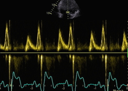
Ultra high frame rate tissue Doppler (about 1200 FPS) from the base of the septum a normal subject. The timing is evident, with ECG starting first, then the pre ejection velocity spike starting about 23 ms later, and then the mitral valve closure about 30 ms after this. This recording is from the septum, and as can be seen, in the septum there is a second spike before ejection starts. It can be seen to repeat from beat to beat. This was not present in the lateral wall.
The findings were later confirmed by a simple study with transfer of valve motions from Doppler flow recordings to tissue Doppler (72). This method is slightly less accurate, both because of the lower frame rate, and as there is some heart rate variability when valve clicks are transferred from other cycles.

Valve closures by valve clicks, and openings by onset of Doppler flow, to the right transferred to the analysis window for tissue Doppler to the left. Relations between timing of tissue Doppler motions and valve motions are typical: Q to onset pre ejection spike (EMD) was about 25 ms, duration of the pre ejection spike about 50 ms, and MVC to end pre ejection spike (ms) about 10 ms.
However the findings were close; Pre ejection spike:
Thus, pre ejection spike is not isovolumic contraction. This rather absurd explanation is a contradiction in terms, as it is present both in the septum and lateral wall, it must necessarily correspond to a volume reduction, which means that the phase is not isovolumic at all. Still, there were some publications on both isovolumic velocity and isovolumic acceleration as contractility measures based on this erroneous concept, as discussed below.
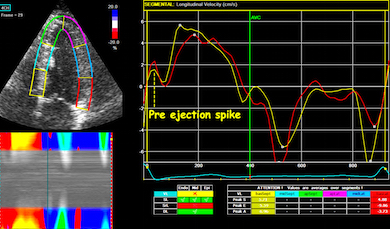
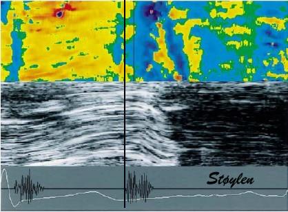
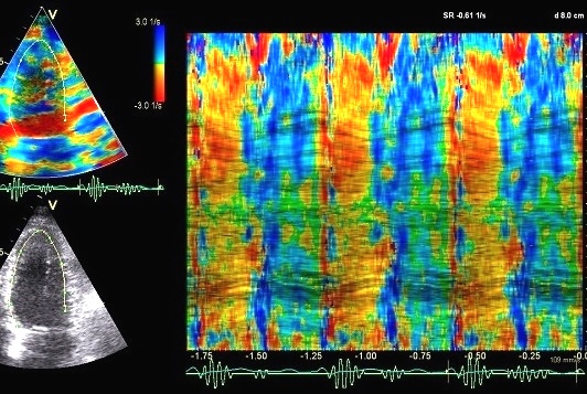
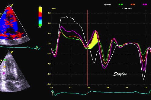
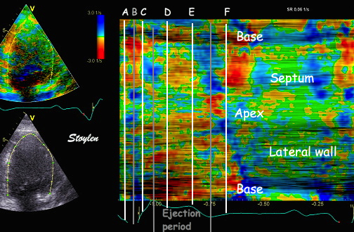
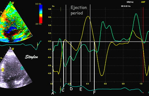
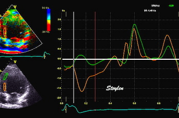
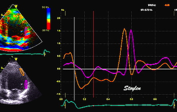
The pre ejection shortening has so short duration, that it is most readily demonstrated by strain rate rather than strain.
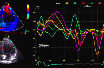
Pre ejection strain rate, active contraction can be seen to be simultaneous in both walls and in both basal and apical level, and to occur before MVC.
In 1973 by phonocardiography (115), and in 1978 by radioopaque markers (116) the ventriculoatrial crossover was demonstrated to occur ca 40 ms before MVC, demonstrationg that this is the onset of thesion buildup, i.e. that this pre ejection motion is active contraction.
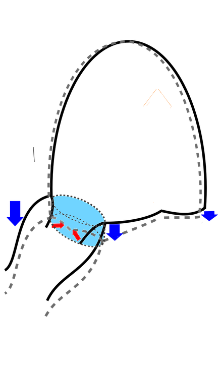
The finding of mitral ring motion in both walls, must mean that this is a real volume reduction of the LV (72), again indicating that this is active contraction. Even without mitral flow, the displacement of the mitral ostium will exclude (atrialize) a small volume from the ventricle:
The apical ring motion is equivalent to a longitudinal shortening, as shown by the strain rate above, and thus a volume reduction, not by flow, but by exclusion of a small volume by the ring motion while the mitral valve is still open.The ring motion will also displace the mitral leaflets towards the base and middle, as they move in the blood. However, the main mechanism for MVC seems to be intraventricular flow as discussed later.
This volume reduction before MVC was also demonstrated experimentally in dogs by conduction catheter, and was shown to be ca 4.2% of EDV (117).
The presence in both septum and lateral wall, and the fact that both walls show negative strain rate (72), as well as the concordance with the known electrophysiology (111 - 113), makes it also very probable that the pre ejection spike is active contraction, and shows the true electromechanical activation, by the left anterior and left posterior bundles.
The pre ejection motion, is thus a contraction, representing a shortening before MVC, meaning at a load of atrial pressure, i.e. near unloaded. Peak pre ejection (72):
Peak pre ejection | Septal | Lateral |
Velocity (cm/s) | 3.59 (1.56) | 3.55 (1.58) |
Strain rate (s-1) | -0.77 (0.61) | -0.66 (0.38) |
Standard deviations in parentheses.
Could this be a measure of contractility?
|
|
Isotonic isometric twitches. The peak tension development is slightly after onset of contraction, | Pre ejection velocity spike occurs before MVC, and thus occurs at the level of atrial pressure, as close to an unloaded situation as one gets. |
Although some papers have been published with "isovolumic acceleration" as contractility measure, it isn't.
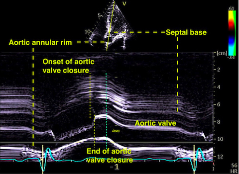
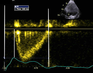
Logically, the MVC should be at the abrupt stop of the pre ejection displacement, i.e. where the velocity trace crosses the zero line after the spike due to the sudden increase in resistance to movement at the closure ov the valve as the cusps stay in the stationary blood stream :
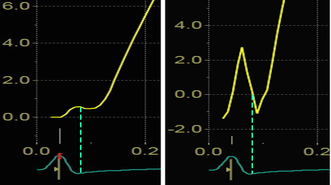
Blown up image of the pre ejection period, displacement to the left, velocity to the right. The logical time for the MVC is when the apical displacement stops abruptly. This is equivalent with the velocity spike retuning to zero, as can be seen with the relation to ECG. As we see, there is a slight initial velocity, and then a break point in the velocity curve, concomitant with the onset of shortening as seen by the displacement curve, corrsponding to the second spike as seen below.
Thus it's the MVC that is actually terminating the pre ejection longitudinal motion /volume reduction.
An experimental study, where the MV was stented open, confirmed this, showing that while shortening started at the same time in the stented situation, the motion (and strain) continued directly into the ejection phase, without the abrupt stop after pre ejection velocity, showing that the start of pre ejection shortening is the true electromechanic activation, while it is the MVC itself that terminates the pre ejection spike (117):
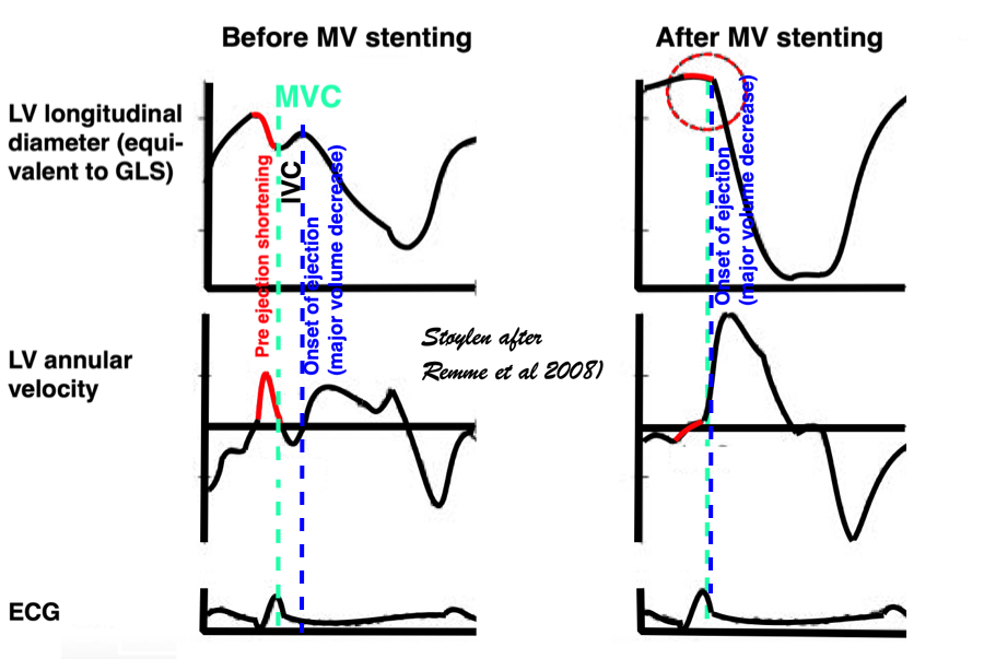
Representation of the findings in the experimental study, showing that as onset of contraction results in shortening, this is interrupted by MVC (onset of IVC), and the velocity spike returns to zero. When mitral valve is stented, this results in a smooth non-interrupted transition to ejection velocities, so the pre ejection strain and velocity (red part of curves) are nearly obliterated, and the onset of the ejection phase the major volume rediction seen by the major downward stroke of the strain curve and the upward stroke of the velocity curve) is starting at the point of the previous MVC, thus the ejection phase now starts at the onset of what was IVC without the stent..
Thus, the pre ejection velocity or strain rate spike is not in accordance with the physiological expectations, and peak protosystolic velocity is not a close measure of maximum unloaded shortening velocity / rate.
The reasons for this may be that as an event of very short duration;
The main point is that the peak protosystolic velocity or acceleration is not a contractility measure.
It has been suggested that the pre ejection annular motion is the mechanism for MV closure (117), the apical motion of the annulus on the stationary blood forcing the valves in the basal direction. However, the basal mitral leaflet motion is greater than the apical motion of the annulus, so this is insufficient to explain the closure. In addition, this hypothesis doesn't take the intraventricular flow into consideration.
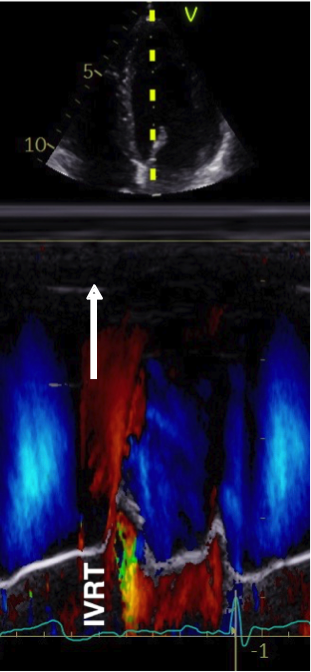
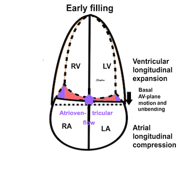
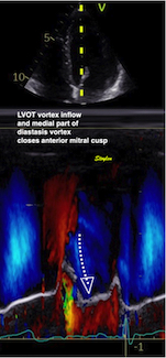
During pre ejection, concomitant with the QRS, there is an intraventricular vortex that stems from the early and late filling vortices.
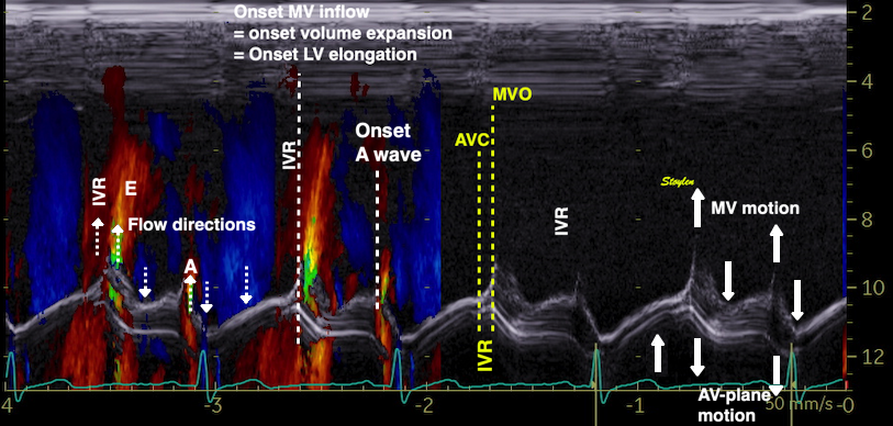
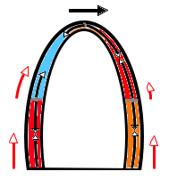
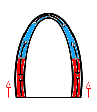
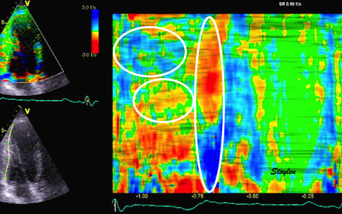
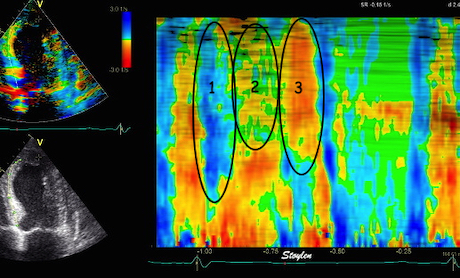
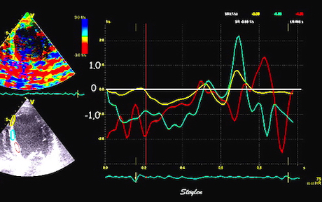
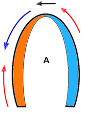
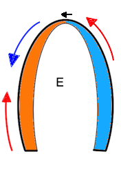
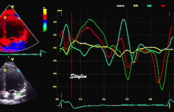
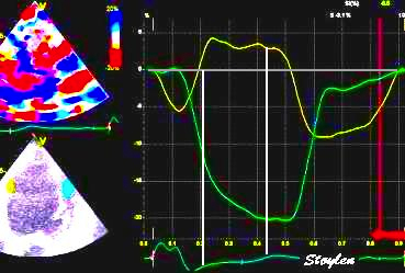
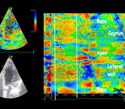
At the end of diastolic filling, the flow in the ventricle consists of a vortex formed by merger of the vortices from the early and late filling phases as discussed later. This vortex is counterclockwise seen in the traditional 4-chamber view, with basally directed flow along the septum, and apically directed flow along the lateral wall (118, 119).
|
|
|
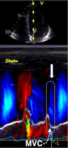
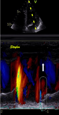
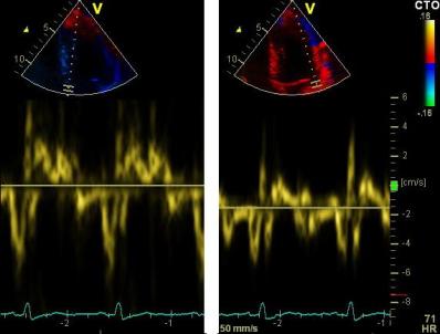
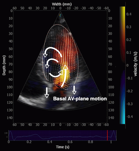
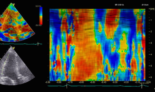
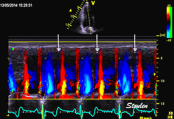
Septal colour M-mode showing basally directed flow along the septum during PEP. It can be seen to start at the beginning of MV closure, and is directed towards the anterior mitral leaflet. | Vector flow imaging, showing the intraventricular counterclockwise vortex during pre ejection, already before MVC. The finding is consistent with the colour M-mode findings. Image courtesy of Annichen S Daae. | Lateral colour M-mode showing apically directed flow along the lateral wall during PEP. |
The vortex is the end result of the diastolic filling (118), as discussed later. The basally directed flow along the septum will contribute to two mechanisms:
The true isovolumic contraction time (IVC) is defined from MVC to AVO, and MVC is defined by the true valve closure, while the AVO is marked by the start of LVOT flow:
As shown above, MVC is at the end of pre ejection tissue velocity:

Thus, in this phase there is no volume change, and, hence, no deformation. This phase it on the other hand, the period of most rapid pressure rise, peak dP/dt, which occurs during IVC, close to the AVC (121). This represents the most rapid rate of force development (RFD). Peak dP/dt can be measured from flow velocity if there is a small MR (122).
|
|
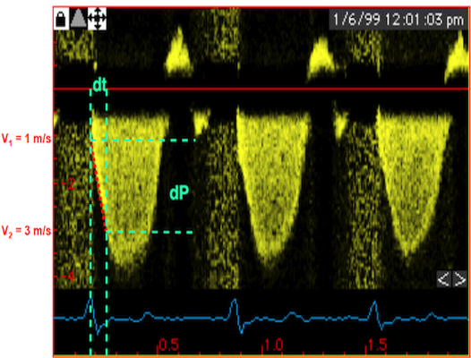
Peak rate of pressure rise, which is the closes correlate to the rate of force/tension development. This occurs during IVC | dP/dt can be measured by the velocity increase, if there is a small MR, too small for generating a pressureincrease in the atrium. It is customary measured between 1 and 3 m/s, which is equivalent to a pressure increase of 32 mmHg, and the dP/dt becomes a function of the time interval between then, and is used as proxy for peak dP/dt |
As it occurs before AVO, it is not afterload dependent (121), and is a useful invasive index of contractility. However, as seen fom the length force relation above, this maximal force measure is not preload independent.
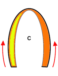
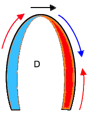
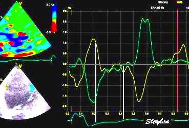
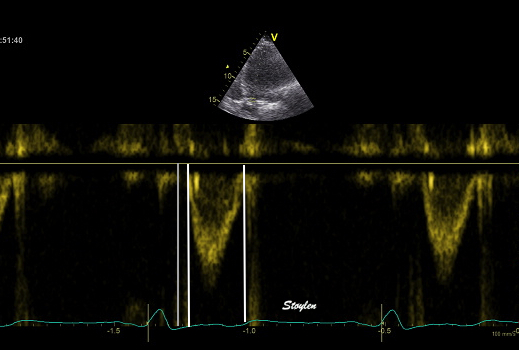
During pre ejection, the vortex is seen to persist after MVC, and the septal part aligns with left ventricular outflow (118). This adds momentum and kinetic energy to the ejection flow.

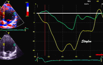
Septal colour M-mode showing basally directed flow along the septum during PEP. It continues until AVO, adding momentum to the ejection, while the lateral, apically directed part of the vortex seem to attenuate.
This means there is a momentum towards the base, aligned with the LVOT even before the AVO. The velocity momentum is equivalent to a partial pressure gradient, and thus contributes to a small reduction in afterload, facilitating the ejection, by conservation of kinetic energy from filling in the vortex.
Vorticity is a measure of the rotation of the blood around each point in the image at one timepoint in the cardiac cycle and is a measure of the complexity of the blood flow. The unit of vorticity is Hz. The time trace of vorticity is found by averaging the region of interest (the LV). In our application, this is calculated by the curl or momentum of
the blood velocity field.by the formula:
As it is measured over a 2D area, it may differ from volume based calculations. The main interest is in the changes in vorticity during the heart cycle, and the relation to the kinetic energy.

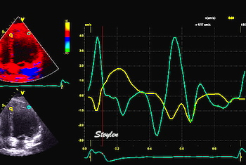
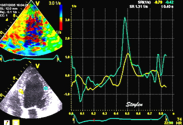
Vorticity plot, showing that vorticity peaks during pre ejection and declines during ejection, despite the ejection showing higher kinetic energy. A reasonable assumption is that kinetic energy is transferred from the vortex to kinetic energy in ejection flow. Images courtesy of Morten S Wigen.
Vorticity is a quantitative measure. Mean vorticity was found in our study to be 10.0 Hz (9.2 - 11.1) in diastole and 8.6 (7.8 - 10.1) in systole (118). Again vorticity will probably differ between applications. The qualitative description can be seen from the 2D vector flow above, reasoned from the colur flow M-mode above, and even seen from the pulsed wave Doppler flow:
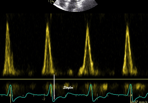
|
|
|
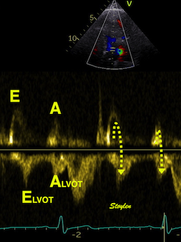
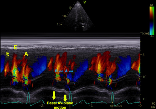
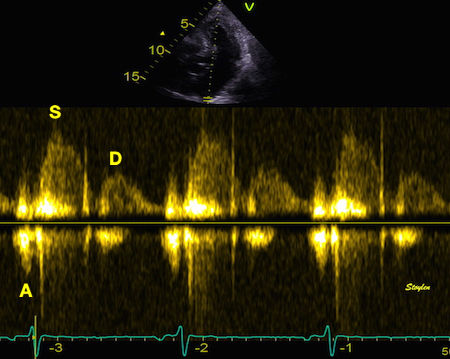
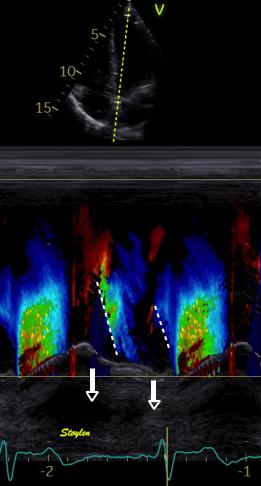
The vortex is present in diastasis, but increases during late filling. Image courtesy of Annichen S Daae | pw Doppler, showing that both early and late inflow are diverted into the LVOT by a slight delay, which visualises the vortices related to the inflow. | This diversion is related to the basal motion of the AV-plane, as seen by the colour M-mode. |
Thus, qualitative clues to the vorticity are present. The presence of vortices in large parts of the heaqrt cucle, is assumed to conserve kinetic energy form one phase, to be utilised in the next, as discussed under the different phases.
It is evident that the kinetic energy is closely related to flow velocity.
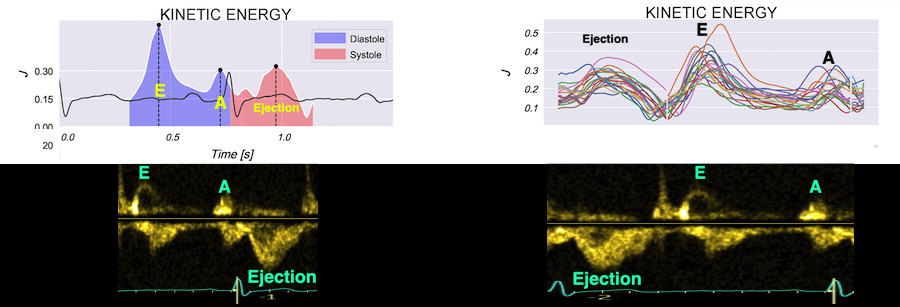
The energy unit is J/m, as we do an integration of 2 dimensions only. As we see, there is a close correspondance between the velocity curves and the energy traces.
The kinetic energy per volume of blood is given by the formula:
![]()
where is the density of blood and v is the flow velocity. Blood speckle tracking allows for estimating the total energy, not only the velocity components along the ultrasound beam as in Doppler. But we do not have full volumetric data, we integrate over a 2-D region (the left ventricle), with the resulting unit of J/m.
![]()
The mean energy is found in our study was 0.21 (0.18 - 0.25) J/m in systole and 0.20 (0.17 - 0.23) J/m (118). The values will differ between applications, as the spatial algorithms will vary, and the unit J/m, which is the 2D measure differs from the true volume measure.
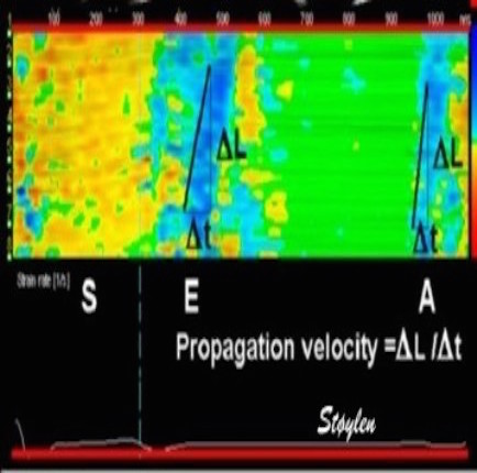
When inflowing blood is diverted into a vortex, the kinetic energy is conserved, to the degree that velocity is maintained. The vorticity is thus a measure of energy conservation. Peak vorticity can be seen to coincide with, but slightly later than the peak vortex inflow in LVOT:
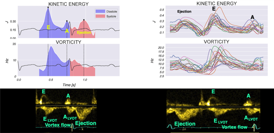
There is some kinetic energy at the onset of early filling, which is expected from the mechanics of the IVR. Vorticity at end ejection IVR is at a minimum, although not absolutely zero, some vorticity generated at end ejection is still present. As we see, there is a close correspondance between the velocity curves and the energy traces, and between the vorticity curves and the vortex inflow in LVOT.
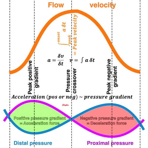
Flow velocity depends on the pressure gradients.
Pressure gradients can be estimated from the flow velocity field:
![]()
![]()
is the density of blood, about 1060 kg/m3 , (vx, vy) is the velocity vector and
is the blood viscosity; about 0.004 Pa/s.
Intraventricular pressure gradients were calculated along a manually defined path from base to apex (118):
![]()
Of course, calculating pressure gradients from flow, doesn't explain flow pattern, as the pressure gradients are derived from the flow pattern at the outset. Thus, thie explanation would be tautological, it is just a description of flow velocity in terms of pressure.
Positive intraventricular pressure gradients (pressure increase) towards the apex will accelerate blood flow towards the base/LVOT (ejection), and decelerate blood flow towards the apex (inflow). Negative intraventricular pressure gradients (pressure decrease) towards the apex will accelerate blood flow towards the apex (inflow) and decelerate blood flow towards the base/LVOT (ejection). There is a correspondence between velocity, as velocity increases, pressure falls, as velocity decreases, pressure increases.

Pressure gradients derived from flow velocities, top mean values, bottom all individual traces. The positive gradient means pressure increases from base to apex/decreases from apex to base, the negative gradient the opposite; pressure increase from apex to base/decrease from base to apex. This means a positive gradient is a driving force for flow from apex towards the base (LV outflow), and a decelerating force for flow from the base towards the apex (LV inflow), a negative gradient is a driving force for flow from the base towards the apex (LV inflow) and a decelerating force for from apex towards the base (LV outflow). Ejection has a biphasic pattern with positive - negative gradient, both early and late filling has the opposite biphasic patternnegative - positive gradient. Images courtesy of Solveig Fadnes and Morten S Wigen
Thus, there is also a dynamic interplay between potential energy (pressure) and kinetic enery (flow velocity) in addition to the interplay between vortex energy and laminar flow energy throughout the heart cycle as well.
The relation between flow acceleration and deceleration and pressure is also discussed below.
With high frame rate, we found that the pre ejection spike was double in the septum, but biphasic in the lateral wall. The second spike, however, was after the MVC, so this is not the atrial rebound and then the pre ejection contraction, tyhe first spike is bilateral and represents the pre ejection contraction, the second being in IVC. This is also evident as the double septal spike is seen even in atrial fibrillation.
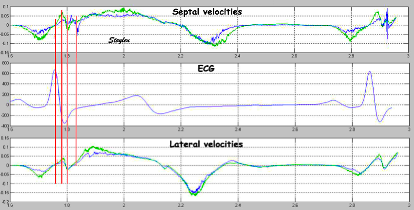
Simultaneous recirdings with UHFR TDI from the septal (top) and lateral (bottom) base. Each recording consists of two velocity curves from two points along the Rx beam, with a distance of 1 cm. Green is the most basal. Thus, the offset between the curves represent the strain rate. The second spike seen in the septum, is not present in the lateral wall, where there is a negative velocity instead. The secons spike is after MVC, i.e. in the IVR. As this motion is reciprocal in the two walls, it represents a rocking motion, not a true volume reduction..
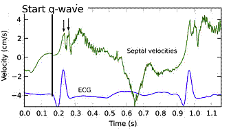
Ultra high frame rate tissue Doppler from the base of the septum a subject with atrial fibrillation. Even with no atrial activity, there is the same pattern of double velocity spikes, showing both to be ventricular in origin.
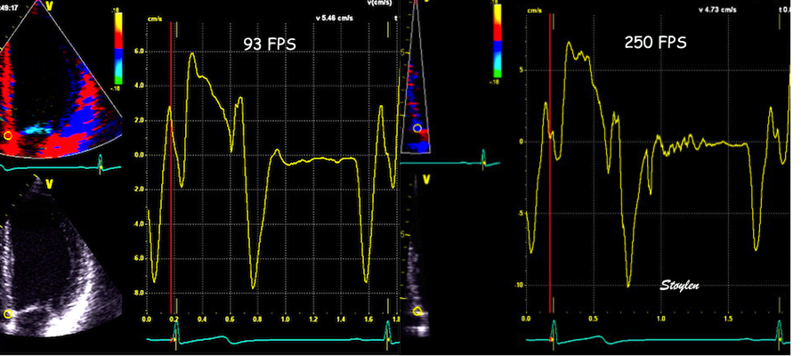
Tissue Doppler from basal septum of healthy subject. at 93 FPS, only one pre ejection spike can be seen, due to undersampling. By using narrow sector and maximum frame rate, it is possible to achieve 250 FPS, and here the pre ejection spike is evident. (That this is not a phenomenon of random noise, as the double spike is reproducible at the start of the next cycle.
Thus, the double spike is not the atrial rebound followed by the electromechanical activation, by the electromechanical activation followed by the IVC rocking motion. The physiological significance of this, however, is uncertain.
The apex beat can be felt through the chest wall by clinical examination. This, in itself, shows that the apex moves towards the chest wall in systole, although only a minimal amount.
The motion was first demonstrated by apexcardiography (10)
|
|
|
The apex beat, shown here in an apexcardiogram recorded with a pressure transducer, demonstrating that the beat is a systolic event. (Image modified from Hurst: The Heart). | But the B-mode and M-mode echoes shows the apical motion towards the chest wall to be minimal | |
The apex beat can also be demonstrated by M-mode and tissue Doppler:
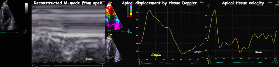
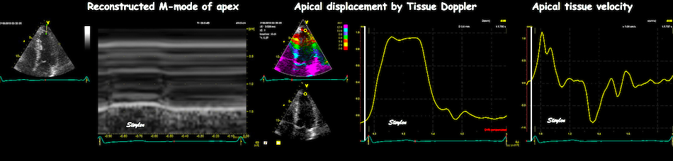
Apex beat from two different healthy subjects. Left: M-mode, middle apical displacements (from integrated velocities), and right: apical velocities.
The apex beat is seen from the pre ejection period, through the ejection. It seems logical that the apex beat is caused by the rereaction from the ejection, ocurring in the opposite direction. However, the onset of the apex beat precedes ejection.
|
|
|
Resolving the motion, we see that the anterior motion in this case starts even before the start of QRS (A). (The motion seen in the displacement curve starts below zero because the tracking is set at zero by the ECG marker). Peak forward velocity (B1) is just after the QRS, while the motion stops in systole (B2), but the apex remains in the anterior position. At end systole (by T-wave in ECG), there is the start of backward motion (C), and the apex returns to the diastolic position at D. | Comparing the apex tissue velocity with LVOT flow (aligned by ECG), both start and peak apical velocity occurs before start ejection, but continues into ejection. In this case, even a second peak may be seen starting at start ejection, indicating a second impetus from ejection recoil. | And for illustration the relation between apical displacement and ejection. Apical displacement starts before ejection, and then continues into ejection, and maximal apical displacement is close to peak ejection velocity. The apex remains pressed to the chest wall during most of ejection, until the flow velocity is so low as to not generate sufficient recoil pressure, while the full return to diastolic position is somewhat later. |
And actually coincides with the pre ejection velocity.
|
|
Comparing this with basal velocities, we see that the anterior motion of the apex starts in the pre ejection phase. The basal pre ejection spike, however, reaches peak before the apex velocity, which peaks close to the time of start ejection (B), by the tissue Doppler curves. Backward apical motion starts a little before end ejection (C), while end of backward apical motion is well within the early filling phase (D) | Relation between apical and basal displacement shows the same. |
while there is initial pre ejection contraction in the base and midwall, resulting the MVC as discussed above, this would tend to pull the apex away from the chest wall as there is no recoil force at that point. However, there is an impact from the blood coming nto the ventricle, which pushes the apex towards the chest wall already before the ejection as seen by the tissue Doppler. In stretch, this should mean that there has to be initial stretch of the apex during the pre ejectioon, simultaneous with shortening of the midwall and base.During early ejection there is thus an acceleration of the ventricle due to recoil from ejection.
The momentum of ejection is the mass of 2x SV (From the RV and LV), x mean outflow velocity. The opposite momentum is the same mass (Outer AV-plane area x AV-plane motion), but the velocity of the AC-plane is ony ca 1/10th of the blood velocity, so there is a surplur momentum pushing the nentricles towards the chest wall.
The first temporal derivatives of these parameters are
The spatial derivative of flow is
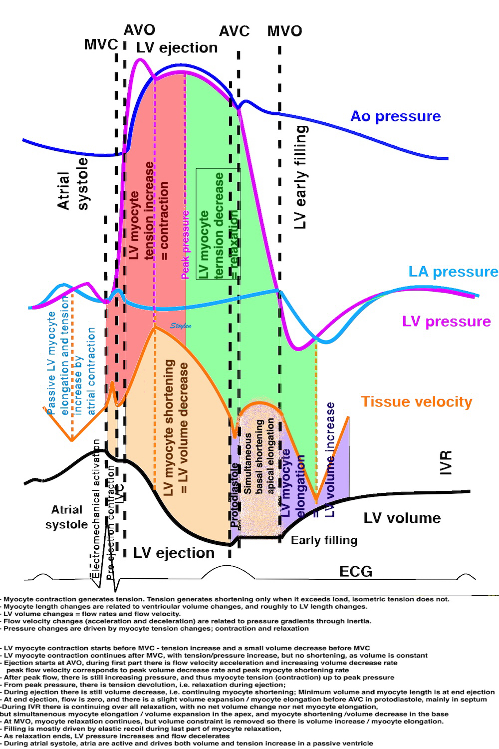
There is not a direct correspondence between contraction (tension) and shortening, nor between relaxation (tension devolution) and fibre lengthening.
As discussed above, all measures of systolic deformation is the result of fibre shortening, and fibre shortening is the result of tension versus load, and thus are not load independent. But the contraction tension is somewhat related to all measures of ejection.
As discussed above, the onset of electromechanical activation is the pre ejection.
The ejection phase, is the phase where blood is ejected, and thus the ventricular volume is decreased. The flow is the rate aof volume decrease, and thus the ventricular volume decrease equals the ejected volume.
As discussed above, electromechanical activation is marked by the pre ejection velocity spike, even before MVC, and long before AVO. During pre ejection, there is isometric contraction leading to tension increase, and thus to pressure increase.
Onset of the major shortening occurs with AVO (72, 121), and is thus a marker of onset of ejection, meaning the onset of the major volume reduction event during systole, but not of electromechanical activation. The onset of rapid upstroke velocity by colour tissue Doppler was found to be 3.8 (10.2) ms after onset of flow in the septum, and 1.0 (17.3) ms in the lateral wall (72). Thus, this marks AVO, and not electromechanical activation.Onset of rapid motion towards the apex, or rapid negative strain rate, are both markers of the onset of the rapid volume decrease, aka the ejection, aka AVO.
During ejection, both longitudinal shortening (MAPSE, peak S', GLS and global strain rate) are related to decrease in ventricular volume, and thus to fibre shortening. Flow is the rate of volume, and thus is another way of expressing volume change, and thus also a measure of fibre shortening. Thus, all measures are related to stroke volume, and to fibre shortening, and all are afterload dependent.
Ejection starts with AVO, which starts the volume decrease, and the flow in LVOT. Flow is the volume rate: volume per time Q = V/t and is usually given in litres per minute. This means that the flow also is the rate of volume change, during ejection thus the volume decrease rate. Even though the traditional wiggers diagrams show peak rate of volume decrease at AVO, this is not the case, as flow studies have shown peak flow (aka peak rate of volume decrease) to occur later, but before peak pressure (104). This has also been confirmed by direct volumetry (263).
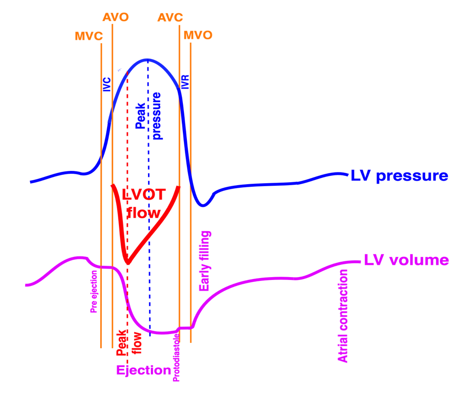
Diagram showing the pressure-volume diagram together with the LVOT flow curve as above, showing the early peak flow, which coincides with the steepest part of the volume curve, )as expected when flow is the rate of volume decrease) occurring before the peak pressure.
It is a myth that blood always flows "downhill" down a pressure gradient, meaning from higher to lower pressure.
The truth is that flow is accelerated down a pressure gradient. This means that there is flow along a positive gradient as long at it's being accelerated, but there may be flow against a positive gradient as long as there is a positive velocity that is being decelerated.
|
|
The pressure gradients are the accelerating force for blood. With a positive gradient, blood is accelerated, with a negative gradient, flowing blood is decelerated. Acceleration is the temporal derivative of velocity, velocity the temporal integral of acceleration. | Both during ejection and during early and late filling is the pattern positive-negative gradient, with peak velocity at pressure crossover. |
Acceleration means converting potential (pressure) energy to kinetic energy, while deceleration means pressure recovery.
|
|
The curves show that only during flow acceleration to peak flow velocity is LV pressure actually higher than the aortic pressure (positive gradient), during the rest of ejection is the pressure gradient negative. However both LV and aortic pressures continue to increase, as a function of continuing contraction generating increasin myocyte tension. This work, however, generates increasing aortic tension, maintaining the negative gradient. | Flow velocity curves are consistent with this., showing a short acceleration phase, a longer deceleration phase. |
During ejection, there is a positive pressure gradient out of the LV only until peak velocity, after that, meaning almost the whole ejection phase the pressure gradient is negative, and the flow velocity is seen to be decelerating. (104, 267, 268)
Doppler gives flow as a velocity. This means the velocity shows how rapidly the blood volume moves along the path, the distance per time v = d/t and is given in m/s. The velocity says nothing about the amount of blood, however. Flow is the volume rate: volume per time Q = V/t and is usually given in litres per minute. But given constant orifice area, any changes in velocity will be proportional to the change in blood volume flow, , showing that there is a fundamental relation between cross sectional area of the flow, and the velocity:
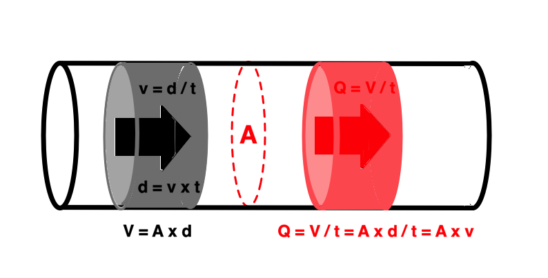
Relation between velocity and flow with constant flow velocity. In this case, the velocity is distance / time v = d / t. During this time interval the distance times cross sectional area defines a volume V = A × d, which is the volume circumscribed by the motion with the velocity v. Flow (volume rate, volume per time) during the same interval t is Q = V / t, so Q = A × d / t = A × v.
This, however, holds only for constant flow velocity. Blood flow is pulsatile, but the fundamental equations of motion still hold:
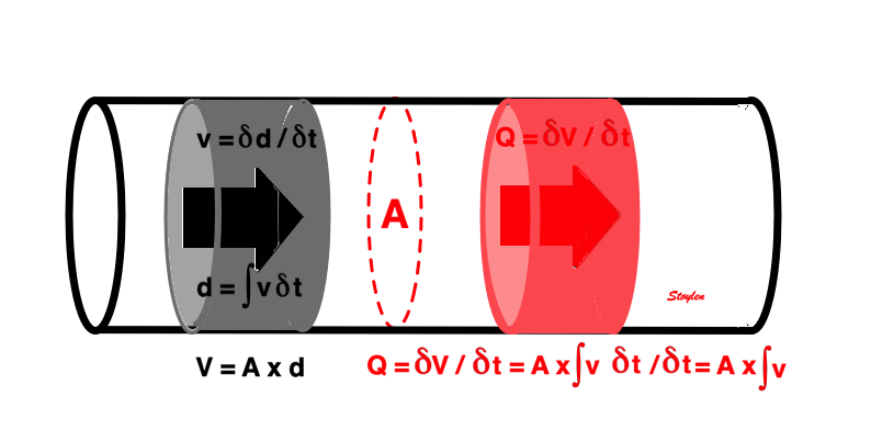
Relation between velocity and flow with constant flow velocity. In this case, the velocity is distance / time v = d / t. During this time interval the distance times cross sectional area defines a volume V = A × d, which is the volume circumscribed by the motion with the velocity v. Flow (volume rate, volume per time) during the same interval t is Q = V / t, so Q = A × d / t = A × v.
Thus, flow = velocity × cross sectional area. In variable velocity, like the pulsatile flow in circulation, the flow equals the velocity integral times the cross sectional area. The integral can be obtained by the area under the velocity curve.
|
|
| |
Tracing the flow velocity curve by pulsed Doppler in LVOT through one heartbeat, gives the velocity time integral by the area under the curve. The LVOT diameter, can be measured in the B-mode. | The velocity time integral is the distance d, that somethin moving with the velocity of the traced curve moves, the stroke distance. The area A of the LVOT (assuming a circular cross section) is given by the measured LVOTdiameter. Thus, the volume of the cylinder given by d × A, equals the stroke volume. |
As long the area is constant, flow velocity and flow are proportional, and simultaneous. This means that flow velocity will reflect the flow. If area changes, there will be a discrepancy between flow and flow velocity, as flow remains constant, while flow velocity increases.
In a continuous channel, flow is contiguous, and must be the same across every cross section, i.e. independent of cross sectional area:
As the area A1 is larger than A2, in order to push the same amount of blood through A2, the velocity v2 must be higher than v1. As the flow is the same, and given by A×v for continuous, and A×VTI for pulsatile flow, the ratio of velocities / velocity time integrals is the inverse of the ratio of areas. This is the continuity equation. | Using the continuity equation, as the LVOT diameter (and area) is known, tracing the VTI of the LVOT flow (pw Doppler to do it in the correct level) as well as the VTI through the valve (cw Doppler). The VTI equals the stroke length, and the stroke length times the atra, equals the stroke volume. As the stroke volume is constant, the two cylinders have equal volume, and thus, the valve stenosis area (AVA) can be calculated by AVA = LVOT area × VTILVOT / VTIAO |
This demonstrates that as contiguous flow needs to be constant, flow velocity will vary with the cross sectional area, and thus will not be representative of flow, unless area is taken into account.
The continuity equation for aortic valve area has been validated against the Gorlin formula (233):
Fundamentally, both velocity and pressure represents energy. The potential energy in a fluid under pressure, is given by E = P × V, while the kinetic energy is E = ½ m v2. But this means that when velocity increases, this kinetic energy has to be recruited from somewhere, which is the pressure energy. Thus, as velocity increases, pressure has to drop:
As velocity increases for the same volume that passes point 1, also must pass point 2, the increase in kinetic energy pressure is recruited from the pressure energy. Thus, there is a pressure drop from 1 to 2. The full equation for the acceleration of the fluid is given in the Bernoully equation. However, it has been shown that both the flow acceleration part and the friction parts are so much smaller than the first part (which is the basic energy difference), and may be ignored. Thus, the modified Bernoully equation relates pressure differences to the square of velocity differences. And if v2 is much smaller than v1, the modified equation may be simplified even more. And of course, the simplest form, is still an acceptable approximation if P2 is much lower than P1.
The simplified Bernoully equation has been shown to be valid for pressure gradients across mitral stenosis (234, 235), aortic stenosis (236), and estimation of RV pressure from tricuspid regurgitation (237).
As discussed above, as flow converges towards a stenosis, there is little friction, meaning that there is laminar flow towards the stenosis. When flow has passed the stenosis, and into a receiving chamber where there is larger area, the velocity will decrease again. However, this may have different consequences. If there is perfectly laminar flow after the stenosis, the friction element is still so small, that the kinetic energy reverts to pressure: there is pressure recovery, and the pressure rises to the pre stenotic level. Doppler measurement will still measure the maximum pressure drop, and so will a manometer placed at the narrow part, but manometers before and after the stenosis will not register pressure drop.
On the other hand, if the flow is not perfectly laminar, there will be turbulence after the stenosis, resulting in frictional energy loss, and the velocity will decrease without restoring pressure energy, i.e. the energy is lost, and there is not pressure increase after the stenosis. In that case, there the Doppler gradient may be a true measure of pressure drop.
Full, partial and zero pressure recovery. The pressure drop corresponding to the velocity increase, is ![]() Pmax, the maximum pressure drop, given by P1 - P2. The net pressure drop through the stenosis,
Pmax, the maximum pressure drop, given by P1 - P2. The net pressure drop through the stenosis, ![]() Pnet, however, is given by P1 - P3. Cw Doppler measures
Pnet, however, is given by P1 - P3. Cw Doppler measures ![]() Pmax, (and so will a manometer placed directly into the stenosis, and may thus over estimate the effect of the stenosis.
Pmax, (and so will a manometer placed directly into the stenosis, and may thus over estimate the effect of the stenosis.
Left is perfectly laminar flow through the stenosis. In this case, the post stenotic velocity decelerates without energy loss, and the kinetic energy is converted back into pressure again. Here, there is no net pressure drop through the stenosis. Driving pressure at P1 does not have to be increased to maintain pressure at P3, and the pressure drop at P2 is temporary. It must be remarked, however, that pressure recovery cannot be more than the initial pressure. | In the middle is partial pressure recovery. Some of the pressure energy converted to kinetic energy through the stenosis is lost when the flow velocity decelerates after the stenosis, in the form of turbulence resulting in friction. But some of the energy is recovered to pressure energy again. Thus, there is a net gradient over the stenosis, but this is less than the maximum gradient. The maximum gradient by Doppler will over estimate the net gradient. | Right, there is total energy loss through the stenosis, all kinetic energy due to the velocity increase through the stenosis is lost in turbulence and friction. Thus, |
As discussed above, if pressure measured across an aortastenosis is higher than normal intraventricular pressure, there has to be a net gradient, as the maximum pressure drop has to be positive.
In MR with a large regurgitation and an eccentric jet, the jet will impinge on the atrial wall, and follow the wall. The jet is deflected by the wall. The jet impinging on the wall will increase the pressure along the wall, and this pressure rise will decrease the flow velocity.
Large, eccentric MR, directed towrds the lateral wall, and then deflected along the wall all the way around the atrial roof and septum. The first red flow cvewlocity is the return of the MR, while the second is the diastolic pulmonary inflow jet.
This has been mistakenly been taken as the result of the Coanda effect, and this mistake has been perpetuated in various publications. However, the Coande aeffect is the apparently paradoxical deviation and adherence to a wall that is parallel with, or deviating away from the jet, and stay attatched to the surface, the mechanism is related to the Bernoully effect as explained below.
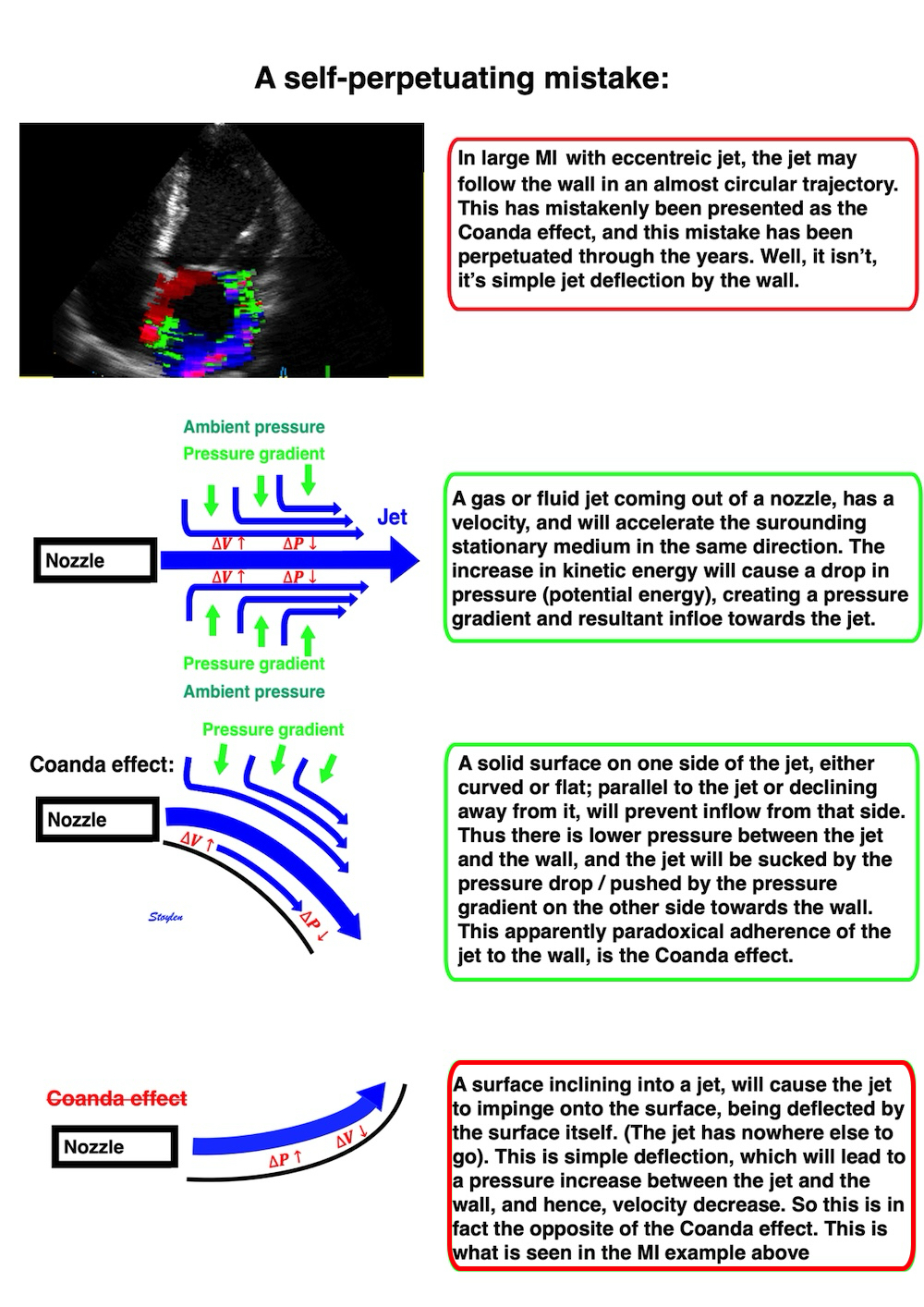
As volume flows into a receiving chamber, (from LA to LV, or from LV to Ao, receiving hambers are elastic, so the compliance decreases with volume received. The concepts of compiance and elastance are discussed above, and the relation to ejection below. As long as compliance and cross sectional area is constant, flow is påroportional with floa velocity, and the volume is proportional with the velocity time integral. However, an elastic receiving chamber decreases the compliance with increasing volume, meaning that for a given pressure increase, the flow volume decreases, or for a given flow volume vthe pressure has to increase.
|
|
for a constant area and compliance, flow volume is proportional with velocity time integral, and equals the temporal derivative of volume. The volume thus equals the time integral of flow. | In an elastic receiving chamber, the compliance decreases (elastance increases) with increased filling. This means that for a given pressure increase, the flow volume decreases with increased filling, or the pressure increases to deliver the same volume. In CV disease, the compliance may decrease, and thus shifts the compliance curve downwards, the elastance curve upwards, decreasing flow volume or increasing pressure. |
Peak ejection performance can be defined as eiter:
As discussed above, the peak rate of ejection (peak flow) occurs early after AVO, and corresponds to the peak rate of volume decrease, aka the peak systolic annular velocity, aka the peak strain rate. Flow and flow velocity has an early peak, The delay after AVO is the time of the acceleration of ejection, and thus as flow iequals the rate of volume decrease, this must be slightly later than the onset of flow as well.
But as has been demonstrated, peak systolic pressure continues to rise until around mid systole (104), which means that peak flow starts to decrease while peak pressure continues to rise. To balance the pressure, peak myocardial tension has to increase as well, so the time of peak tension is the peak of systolic pressure. Why this discrepancy? This is due to the continued distension of the large vessels with the increase in total ejected volume.
So there is an initial increase in flow and rate of volume decrease. Peak flow is related to the contractility, but as shown below, it is earlier than the time of peak tension.
|
|
Peak flow, which coincides with the steepest part of the volume curve, is the peak of volume ejection, but not the peak of LV tension. | During ejection, the volume is ejected into the aorta, which is distended, storing energy in the elastic properties. This distension requires pressure, and is part of the systolic LV work. Thus the tension (and work) continues to increase after peak flow, and the peak tension is at peak pressure. Ejection, continues however, until flow is completely decelerated, at AVC, and thus the maximal aortic distension is at end ejection. The aorta is then contracting again during diastole, acting as a diastolic pump, with energy stored from systole, using this energy as part of the whole pumping cycle. |
The timing of the peak flow, is determined by the crossover between the volume ejection, and the elastic distension of the aorta, which again is a function of both the elasticity and the peripheral resistance, and the magnitude of the peak is in part a function of the timing of the acceleration cutoff. But this also shows that the peak myocardial tension is later than the peak volume decrease/flow/flow velocity.
In fact, as flow is accelerated by a positive pressure gradient, and decelerated by a negative pressure gradient, the cut off of flow acceleration is the point of pressure crossover between the ventricle and the artery, and thus before peak pressure:
|
|
Diagram, showing firstly, that flow is accelerated only during the first part of ejection, at pressure crossover from a positive to a negative gradient, the flow deceleration starts, before peak pressure, but the time of the crossover (acceleration cutoff) itself is a determinant of the peak flow. | As blood is ejected into the aorta, the aorta and large arteries being elastic, they are distended by the volume they receive. This volume is partly a function of the relative ejected volume (during acceleration), i.e. the relation between ejection volume and aortic (arterial) volume. The second factor is arterial compliance; C = |
However, despite the peak flow being early, and flow / flow velocity starting to decrease from peak after AVO, obviously the cumulated flow (which is the true meaning of the integral) and total ejected volume increases untill the end of ejection.
Thus, the peak flow rate is not only a function of contractility and pressure, but also of aortic volume and compliance, and not a "pure" LV measure.
Peak pressure, correspondint to peak tension, however, is obviously related to both stroke volume and aortic volume and compliance.
Peak flow velocity is simultaneous with peak flow, as the aortic orifice is considered constant during ejection. Flow velocity alone says nothing about the amount of blood, however. But given constant orifice area, any changes in velocity (m/s) will be proportional to the change in blood volume flow (l/min), showing that there is a fundamental relation between cross sectional area of the flow, and the velocity. Thus, LVOT flow will show the same early peak as flow recordings, but as shown in the HUNT study, there is not co variabiility between peak S and MAPSE.
Peak annular systolic velocity, S' and peak global SR, are both measures of the peak rate of longitudinal LV shortening, i.e. peak rate of length decrease. As most of the stroke volume is related to longitudinal shortening. they can be assumed to be closely related to peak rate of volume decrease. It can also se a close correspondence in timing of the peaks.
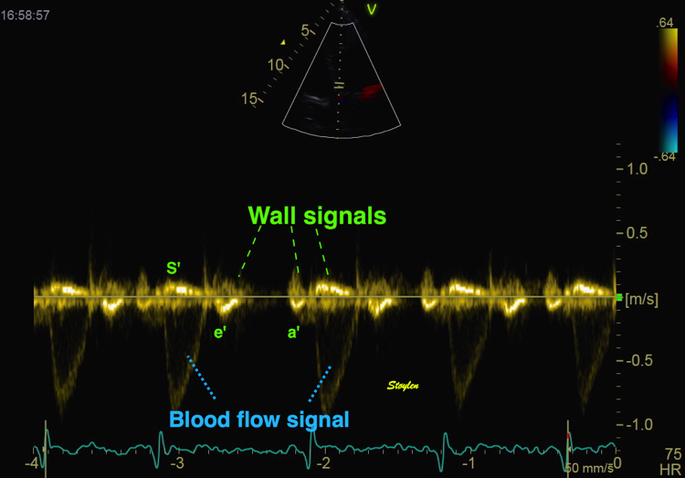
The image shows the early peak of flow velocity in the LVOT. By removing the wall filter and reducing the signal amplitude, the wall signals can be seen as well, and the wall velocity, being proportional with the volume rate, also shows the same early peak.
As the systolic longitudinal shortening is closely related to volume decrease, peak strain rate and peak annular velocity are likewise early events close in timing to peak flow:
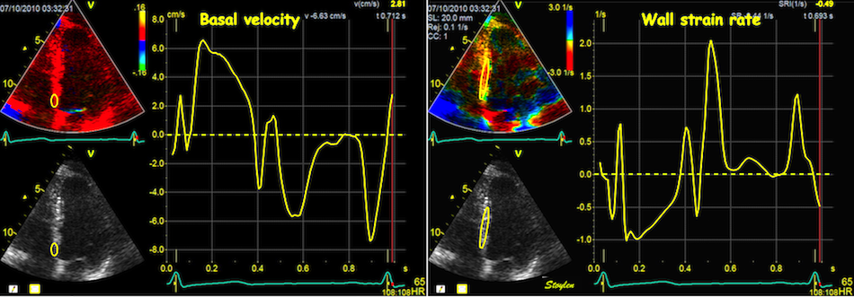
When strain rate is sampled from most of the wall length, the shape is close to an inverted version of the basal velocity curve. In this case, both curves relate to the rate of volume change, and thus to the very early peak flow and the steepest parts of the annulus displacement and strain curves.
|
|
|
Flow velocity of LVOT. This is closely related to flow, showing an early peak during the ejection time. | Tissue Doppler of the mitral annulus from the same subject, showing early peak annular velocity (a measure of peak longitudinal shortening rate), a proxy of volume reduction rate. | Colour tissue velocity from the same subject, with transferred valve openings and closures, showing how early the peak annular velocity is in the ejection time. |
The apex being nearly stationary, the global strain rate (of a wall or the whole ventricle), equals the normalised, inverse value of the matching (wall or the whole ventricle) annular velocity: the annular velocity corresponds fairly closely to the wall strain rate (23).
|
|
As we see, apical velocity is close to zero. | When strain rate (SR) is taken from tissue velocities, the definition is SR= (v(x) - v(x+Δx)) ⁄ Δx where v(x) and v(x+Δx) are velocities in two different points, and Δx is the distance between the two points. If the two points are at the apex and the mitral ring, the apical velocity v(x) ≈ 0, apex being stationary, and v(x+Δx) is annular velocity. Δx then equals wall length (WL), and peak systolic SR = (0 - S') ⁄ WL= (-S') ⁄ WL. |
If the two points are at the apex and the mitral ring, the apical velocity ![]() , apex being stationary, and
, apex being stationary, and ![]() is annular velocity.
is annular velocity. ![]() then equals wall length (WL),
then equals wall length (WL),
thus ![]() and peak
and peak ![]() . It's also evident that the basal velocity curve and the strain rate curve approaches each other's shape when strain rate is sampled from most of the wall length. Thus, a method for peak systolic strain rate is peak annular velocity normalised for wall length.
. It's also evident that the basal velocity curve and the strain rate curve approaches each other's shape when strain rate is sampled from most of the wall length. Thus, a method for peak systolic strain rate is peak annular velocity normalised for wall length.
This means that global peak systolic strain rate and global annular peak systolic velocity are physiologically equivalent.
In the HUNT study, the lateral wall had higher S' than the septum, but the global average of peak annular velocity was the same for two walls (septum and lateral wall) as for four walls (septum, anterior, lateral and inferior wall). The differences between walls in strain rate, on the other hand, was minimal.
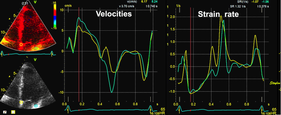
As shown here, peak rate of volume decrease is reflected in both peak systolic velocity and strain rate in this case, as septal and lateral peak velocities and strain rates are simultaneous.
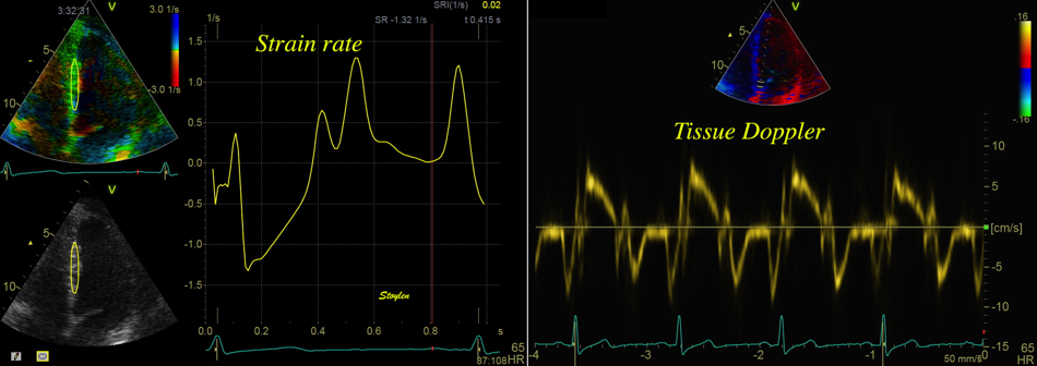
Comparison between colour Doppler strain rate from the septum (left), and spectral tissue Doppler from the mitral ring of the same subject, showing the same curve shape relations as the colour Doppler derived differences as shown above.
Peak systolic measures are still the closest imaging measures of peak ventricular performance, and are basically
Peak flow is also a measure of peak rate of volume decrease, but with Doppler, we measure flow velocity, while flow = velocity x Area. Thus the flow velocity - flow relation is inveresely related to area. Timing of peak flow, however, should be simultaneous to peak S' and SR.
They are positively related to:
And negatively related to
Thus, peak tissue velocity and peak strain rate are all measures close to peak ventricular performance, but load dependent, and occurring after peak rate of force idevelopment, but before peak myocardial tension.
However, they are both early ejection measures of myocardial performance closer to the peak dP/dt and peak myocardial tension, and are measures of the acceleration of blood out of the ventricles.
Peak systolic annular velocity was early related to ventricular function (123 - 126). Peak strain rate was likewise related to inotropy (127 - 129), and correlated better than strain. Weidemann (127 - 128) did not find that SR related to HR, but this might be that HR was increased by pacing, and thus to reduced ventricular filling, and thus concomitant reduction in preload.
In an experimental study with positive and negative inotropy, Greenberg found a correlation between LV elastance and both S' and peak SR (129).
In a human study with Dobutamin, Thorstensen (130) found that all early systolic indices were more sensitive to changes in inotropy, with a 50 - 60% increase in all three measures with Dobutamine (compared to a 13% increase in HR and 14% in SBP), and with an 11 to 15% decrease (compared to a 13% decrease in HR and 22% decrease in SBP) with Metoprolol. None of the responses of the peak systolic indices were significantly different from the others.
Thus, the peak is not only a function of acceleration, but also related to the early cut off of peak flow rate, due to the increase in aortic pressure.
Greenberg found a stronger correlation of LV elastance with peak SR, than with S' (129). This, however, may be due to the open chest model, which increases translational artefacts, which would affect velocities more that strain rate.
In the HUNT study, using the segmental length method by tissue Doppler tracking:
|
|
|
Serch areas for kernel tracking from frame to frame, oraqnge, lo0ngitudinal search areas by tissue Doppler, white areas transverse serch areas for speckle tracking. | Real time tracking of kernels at the segment borders. | Strain rate curves. Green: average of three segments of the wall, blue, curve for each segment |
In addition, we examined the peak systolic annular tissue Doppler values by spectral Doppler (S'), and the S' normalised for wall lengths (19) as an equivalent of strain rate as shown above.
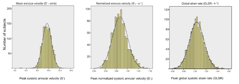
Both strain rate and myocardial velocities were normally distributed (19), and so war S'RV.
The normal values for strain rate and and annular velocities by age and sex were (16, 17, 23):
Annular velocities by sex and age. Values are mean (SD). pwTDI: Pulsed Tissue Doppler recorded at the top of the spectrum with minimum gain, c TDI: colour TDI. Normal range is customary defined as mean ± 2 SD.
S'LV, mean of 2 walls (cm/s) | S'LV, mean of 4 walls (cm/s) | S'nLV, mean of 2 walls (s-1) | S'nLV, mean of 4 walls (s-1) | SRLV mean of 6 walls (S-1) | Peak LVOT (m/s) | S'RV (cm/s) | ||
(pw TDI) | (pw TDI) | cTDI | (pw TDI) | (pw TDI) | Segmental TDI | Single site | ||
Females | ||||||||
< 40 years | 8.8 (1.1) | 8.9 (1.1) | 7.2 ( 1.0) | 0.94 (0.12) | 0.94 (0.12) | 1.09 (0.12) | 1.01 (0.17) | 13.0 (1.8) |
40 - 60 years | 8.1 (1.2) | 8.1 (1.2) | 6.5 (1.0) | 0.88 (0.13) | 0.88 (0.14) | 1.06 (0.12) | 1.02 (0.16) | 12.4 (1.9) |
> 60 years | 7.3 (1.2) | 7.2 (1.2) | 5.7 (1.1) | 0.81 (0.13) | 0.82 (0.12) | 0.98 (0.14) | 1.01 (0.17) | 11.8 (2.0) |
All | 8.2 (1.3) | 8.2 (1.3) | 6.6 (1.1) | 0.89 (0.13) | 0.89 (0.14) | 1.05 (0.13) | 1.01 0.16) | 12.5 (1.9) |
Males | ||||||||
< 40 years | 9.3 (1.4) | 9.4 (1.4) | 7.6 (1.2) | 0.90 (0.14) | 0.90 (0.14) | 1.06 (0.13) | 0.99 (0.17) | 13.2 (2.0) |
40 - 60 years | 8.6 (8.1) | 8.6 (1.3) | 6.9 (1.3) | 0.84 (0.13) | 0.84 (0.15) | 1.01 (0.12) | 0.99 (0.18) | 12.8 (2.2) |
> 60 years | 8.1 (1.3) | 8.0 (1.3) | 6.4 (1.2) | 0.82 (0.14) | 0.83 (0.13) | 0.97 (0.14) | 0.96 (0.18) | 12.5 (2.3) |
All | 8.6 (1.4) | 8.6 (1.4) | 6.9 (1.3) | 0.85 (0.14) | 0.85 (0.14) | 1.01 (0.13) | 0.98 (0.18) | 12.8 (2.2) |
Total | 8.4 (1.3) | 8.4 (1.4) | 6.8 (1.3) | 0.87 (0.14) | 0.87 (0.14) | 1.03 (0.13) | 1.00 (0.18) | 12.6 (2.1) |
Relative SD (%) | 15.5 | 16.7 | 16.1 | 16.1 | 12.6 | NA | NA | |
Annular velocities and strain rates by sex and age. Values are mean (SD). pwTDI: Pulsed Tissue Doppler recorded at the top of the spectrum with minimum gain, c TDI: colour TDI. ll differences between sex and age were significant; all P < .001, but segemntal SR of 2 and 4 walls were not significant, due to too many segments dropped out. Overall standard deviations are given as % of mean in the bottom line, to compare the biological variations between normalized and non-normalized measures. MAPSEn and S′n MAPSE and S′ normalized for LV mean diastolic wall length, respectively. MAPSEn2 and S′n2 normalized for both mean LV diastolic wall length and LV diastolic external diameter, respectively. Abbreviations: GLS = global longitudinal strain; GLSR = global longitudinal strain rate; MAPSE = mitral annular plane systolic excursion; S′ = peak mitral annular systolic longitudinal velocity.
Normal range is customary defined as mean ± 2 SD.
Colour TDI gave lower values than pw TDI as is known since spectral Doppler gives peak values by spectral width, while colour Doppler gives mean values by autocorrelation..
All measures of peak volume change correlated with each other: S' with Global SR by normalised S': unsurprisingly R = 0.87, but alsi with GLSR by segmental tissue Doppler: R = 0.43.
LVOTvmax vs spectral S' : R=0.22, (p<0.001), vs segmental SR 0.17 (0.001), and vs normalised tissue velocity 0.22 (0.001).
But as opposed to SR and S', which declined with age, and correlated negatively respective positively with BSA as described above, LVOTvmax did not correlate with either. As SV is a function of both LVOT velocity (integral) and LVOT area, this indicates that LVOT area is a function of body (heart) size, and that it possibly declines with age. This means that LVOT area is a confounder, and that peak flow velocity in LVOT is not a measure of peak shortening.
- S' declines with increasing age,
- is higher in men than women,
The table shows that:
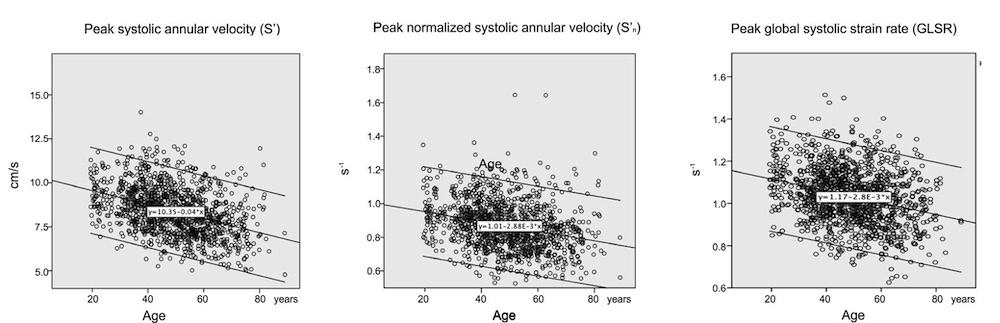
Both velocity and both methods for strain rate shows significantly decreasing absolute values by increasing age.

S', normalised S' and GLSR versus body size (BSA). S' is weakly positively correlated with BSA, while strain rate (both normalised S' and GLSR) are negatively correlated, and with a larger absolute correlation.
the finding that there was no increase in strain rate by increasing body size (BSA), despite increase in S', relates to the fact as elaborated below, that with a larger BSA, the LV is larger, and the SV is larger. However, a larger LV, means that it is both longer and wider (19). As SV is between 60 and 70% dependent on MAPSE (64 - 68), a wider ventricle, will generate a larger SV, even if MAPSE is unchanged. SR, on the other hand only corrects for LV length, and thus induces a systematic error.

Diagram showing that as diameter (and cross sectional area) is larger in a longer ventricle, given the same MAPSE, SV can be higher with the same MAPSE, but GLS will be lower in absolute values
The peak performance of the LV is seen during the first part of the ejection as described above.
|
|
|
Pressure-volume-flow diagram showing peak flow in early ejection, peak pressure in mid ejection and peak volume decrease at end ejection. | Annulus velocity and displacement durves, showing peak velocity early after QRS, and peak displacement at end ejection. | Strain rate and strain curves, showing peak (absolute) strain early after ejection, (the peak is less sharp here, as it is from a smaller part of the wall) and peak (absolute) strain at end ejection. |
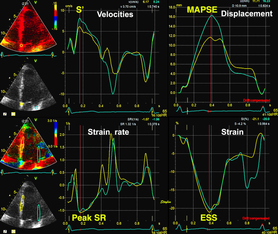
Velocity, strain rate, displacement and strain. S': peak annular systolic velocity, MAPSE: end systolic Mitral Annular Plane Systolic Excursion, Peak SR: peak systolic strain rate, ESS: End systolic strain. All measures are mean of seoptal and lateral for global measures.
Systolic annular velocity, comparison between HUNT3 and 4
HUNT 3 | HUNT 4 | |||||||||||||
Age group | S' Septal | SEM | 95% CI | S' lateral | SEM | 95% CI | Age group | N | S' septal | SEM | 95% CI | S' lateral | SEM | 95% CI |
Women | ||||||||||||||
< 40 | 8.4 (1.0) | 0.071 | 8.26 - 8.54 | 9.3 (1.6) | 0.109 | 9.08 - 9.52 | 20 - 39 | 64 | 8.5 (1.4) | 0.175 | 8.15 - 8.85 | 10.2 (2.2) | 0.275 | 9.65 - 10.75 |
40 - 60 | 7.7 (1.5) | 0.063 | 7.57 - 7.83 | 8.6 (1.6) | 0.085 | 8.43 - 8.77 | 40 - 59 | 357 | 7.9 (1.3) | 0.069 | 7.76 - 8.04 | 9.4 (2.1) | 0.111 | 9.18 - 9.62 |
> 60 | 6.1 (1.2) | 0.112 | 5.88 - 6.32 | 7.6 (1.5) | 0.137 | 7.33 - 7.87 | 60 - 70 | 355 | 7.2 (1.4) | 0.074 | 7.05 - 7.35 | 8.5 (2.1) | 0.111 | 8.28 - 8.72 |
> 80 | 12 | 6.3 (0.8) | ||||||||||||
Men | ||||||||||||||
< 40 | 8.7 (1.2) | 0.109 | 8.48 - 8.92 | 9.9 (1.9) | 0.172 | 9.56 - 10.24 | 20 - 39 | 49 | 9.4 (1.5) | 0.214 | 8.97 - 9.83 | 11.9 (2.1) | 0.30 | 11.3 - 12.5 |
40 - 60 | 8.1 (1.2) | 0.067 | 7.97 - 8.23 | 9.0 (1.9) | 0.104 | 8.79 - 9.21 | 40 - 59 | 284 | 8.3 (1.5) | 0.089 | 8.12 - 8.48 | 10.0 (2.3) | 0.136 | 9.73 - 10.27 |
> 60 | 7,7 (1.1) | 0.093 | 7.51 - 7.89 | 8.4 (1.7) | 0.144 | 8.11 - 8.69 | 60 - 70 | 279 | 7.9 (1.4) | 0.084 | 7.73 - 8.07 | 9.5 ((2.3) | 0.137 | 9.23 - 9.77 |
> 80 | 12 | 7.4 (1.2) | 8.8 (2.5) | |||||||||||
Both studies show decline with age, but the difference in peak values between the two studies is significant.
However, to assess if this difference is sufficient explanation, we looked at S' isolated in the septum, and still found that the values for HUNT3 and HUNT4 were different for all age groups.
There was a slight difference in mean age, but as the age groups are all significantly different, this is not a reason for the differences.
HUNT 3 was acquired in 2006 - 2008, HUNT 4 in 2017 - 2019. Thus the echo populations are two different cohorts. The two cohorts were similar in sex distribution, BMI and BP.
Both normal studies excluded patients with heart disease, diabetes and hypertension.
HUNT3 was taken on GE Vivid 7, and analysed in EchoPAC version BT06, (except strain and strain rate, which was analysed in the proprietary segmental strain analysis software.
HUNT4 was acquired on GE Vivid E95 and analysed on EchoPAC version 203.
The peak values of spectral Doppler are gain dependent, but this was known at the time of HUNT3, so both studies were acquired with the same convention for spectral Dopppler:
- Peak top of the spectrum
- at lowest possible gain not creating drop outs.
But as there were 10 years technical development, image quality may have improved, enabling a lower gainj setting, and thus lower values in HUNT4
there may be other differences as well:
Package size
Analysis window
Use of sliding windows technique
..............
The main point is that older normal values are not applicable to newer hard- and software.
Systolic velocities vary according to site, as shown in the diagram below.
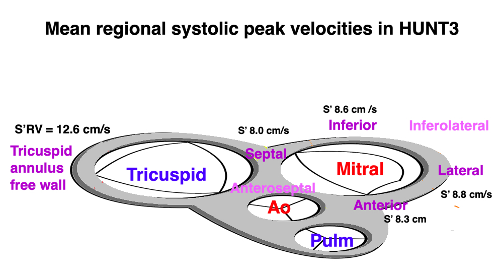
Site variation of systolic velocites (mean values from HUNT3
This is discussed in more details in the chapter of regional MAPSE, but is due to (156):
The
Age | Septal | Lateral | Anterior | Inferior | LV, mean of sep&lat | LV, mean of 4 walls | S'RV |
Females | |||||||
< 40 years | 8.4 (1.0) | 9.3 (1.6) | 9.2 (1.2) | 8.8 (1.2) | 8.8 (1.1) | 8.9 (1.1) | 13.0 (1.8) |
40 - 60 years | 7.7 (1.5) | 8.6 (1.6) | 8.2 (1.8) | 8.3 (1.3) | 8.1 (1.2) | 8.1 (1.2) | 12.4 (1.9) |
> 60 years | 6.1 (1.2) | 7.6 (1.5) | 7.0 (1.7) | 7.4 (1.4) | 7.3 (1.2) | 7.2 (1.2) | 11.8 (2.0) |
All | 7,78 (1.2) | 8.6 (1.6) | 8.2 (1.8) | 8.3 (1.3) | 8.2 (1.3) | 8.2 (1.3) | 12.5 (1.9) |
Males | |||||||
< 40 years | 8.7 (1.2) | 9.9 (1.9) | 9.5 (2.0) | 9.4 (1.4) | 9.3 (1.4) | 9.4 (1.4) | 13.2 (2.0) |
40 - 60 years | 8.1 (1.2) | 9.0 (1.9) | 8.3 (1.9) | 8.9 (1.5) | 8.6 (8.1) | 8.6 (1.3) | 12.8 (2.2) |
> 60 years | 7.7 (1.1) | 8.4 (1.7) | 7.7 (1.8) | 8.2 (1.3) | 8.1 (1.3) | 8.0 (1.3) | 12.5 (2.3) |
All | 8.1 (1.2) | 9.0 (1.9) | 8.4 (2.0) | 8.8 (1.5) | 8.6 (1.4) | 8.6 (1.4) | 12.8 (2.2) |
Total | 8.0 (1.2) | 8.8 (1.8) | 8.3 (1.9) | 8.6 (1.4) | 8.4 (1.3) | 8.4 (1.4) | 12.6 (2.1) |
Annular velocities by wall, sex and age. Values are mean (SD). Pulsed Tissue Doppler recorded at the top of the spectrum with minimum gain, differences between sex and age were significant; all P < .001.
The mean of 2 walls (8.37 cm/s) was slightly different from the mean of 4 walls (8.40 cm/s) (p < 0.001 in pairwise T-test), statistically significant, but totally but uninteresting as the limit for the accuracy of spectral Doppler is only 0.1 cm/s.
Age | Septal | Lateral | Estimated mean of sep-lat | Anterior | Inferior | Estimated mean of 4 | Anteroseptal | Inferiolateral | mean of 6 | S' RV |
Women | ||||||||||
20 - 39 | 7.0 (1.0) | 7.8 (1.9) | 7.4 | 8.3 (2.1) | 7.4 (1.1) | 7.6 | 6.2 (1.3) | 7.2 (1.9) | 7.3 (1.2) | 11.2 (1.6) |
40 - 59 | 6.5 (1.0) | 7.4 (1.6) | 7.0 | 7.1 (1.9) | 7.0 (1.4) | 7.0 | 5.7 (1.2) | 7.2 (1.7) | 6.8 (1.0) | 10.8 (1.6) |
60 - 79 | 5.8 (1.1) | 6.8 (1.7) | 5.9 | 6.2 (1.7) | 6.2 (1.7) | 6.3 | 5.0 (1.2) | 6.8 (1.6) | 6.2 (1.1) | 10.4 (2.1) |
> 79 | 5.3 (0.8) | 6.6 (1.1) | 6.0 | 5.7 (1.4) | 5.4 (0.6) | 5.8 | 4.4 (1.1) | 5.9 (1.5) | 5.5 (0.7) | 10.3 (1.9) |
All | 6.2 | 7.2 | 6.5 | 6.8 | 6.6 | 6.7 | 5.4 | 7.0 | 6.6 | 10.6 |
Men | ||||||||||
20 - 39 | 7.8 (1.2) | 9.3 (2.0) | 8.6 | 9.2 (2.0) | 8.7 (1.3) | 8.8 | 7.1 (1.3) | 9.0 (1.9) | 8.6 (1.3) | 11.2 (1.6) |
40 - 59 | 7.0 (1.1) | 8.0 (2.2) | 7.5 | 7.8 (2.3) | 7.8 (1.3) | 7.2 | 6.0 (1.4) | 7.7 (2.5) | 7.5 (1.2) | 11.1 (2.0) |
60 - 79 | 6.6 (1.1) | 7.7 (2.2) | 7.2 | 7.2 (2.1) | 7.2 (1.3) | 7.2 | 5.5 (1.5) | 7.4 (2.1) | 7.0 (1.3) | 11.1 (1.9) |
> 79 | 6.5 (1.5) | 7.3 (2.6) | 6.9 | 5.8 (1.6) | 6.5 (1.2) | 6.5 | 5.2 (1.0) | 7.3 (3.1) | 6.4 (1.5) | 12.0 (1.9) |
All | 6.5 | 8.0 | 7.4 | 7.6 | 7.6 | 7.3 | 5.8 | 7.7 | 7.3 | 11.1 |
Total | 6.3 | 7.5 | 6.9 | 7.1 | 7.1 | 7.0 | 5.6 | 7.3 | 6.9 | 10.8 |
Values were corrected for the numbers in each age class before averaging for the cohort. The age group > 79 had only 12 persons of each sex, so cinsidering them as representative is meaningless.
CTDI inh HUNT 4 were significantly lower than pwTDI. This is due to the point that cTDI, corresponds to the middle of the spectrum in spectral TDI (modal velocity), while pwTDI measures at the top of the spectrum as discussed in the basic ultrasound section.
The HUNT3 measures by pwTDI S' only in four points, But we found no difference between global S' as mean of septal-lateral and mean of septal-lateral-anterior-inferior (23). HUNT 4, by cTDI, measures in all 6 walls, and the paper only gives the mean of all 6. As seen below, there is a difference, as the anteroseptal values are lower, but not enough to influence the global mean significantly, in line with what we found for MAPSE in HUNT 3 (156).
Despite the differences in method of TDI, the two studies, both studies confirms the general findings:
- S' declines with increasing age,
- is higher in men than women,
- is lowest in the septum and highest in the lv in the lateral wall, and highest over all in the RV lateral wall.
The total performance of the ventricles corresponds to the stroke volume, which is the measure of the total systolic volume reduction, and thus the total ventricular performance, and cumulated myocardial shortening, although a closer approximation would include the pressure (pulse pressure, PP) this work is performed in, i.e stroke work, which is W = SV × PP.
As M-mode was the first echo modality, the fractional shortening of the LV cavity was the first LV systolic functional measure by echo. The fractional diameter shortening is defined as
FS = (LVIDd - LVIDs) / LVIDd
Diameter is conventionally measured to the endocardium, so the fractional shortening is more precisely the endocardional fractional shortening. Thus, it is in fact an one-dimensional version of EF, under the assumption of a symmetrical ventricle without regional dysfunction. It's less accurate than the EF when there is regional dysfunction, as the measured fractional shortening will be generalised to the whole ventricle.

Endocardial fractional shortening, is obviously related to wall thickening, as the wall shortens longitudinally, it will thicken transversely, given the low compressibility of the myocardial volume.

Deformation in systole. Left: end diastolic image, showing the end diastolic length (Ld = L0). During systole, the ventricle shortens with ![]() L, which gives (L = L0 -
L, which gives (L = L0 - ![]() L = Ls). But in order to conserve myocardial volume, the wall thickens at the same time, as shown by the horisontal arrows.
L = Ls). But in order to conserve myocardial volume, the wall thickens at the same time, as shown by the horisontal arrows.
Wall thickening is
WT = (Ws - Wd) / Wd
However, there is also a systolic outer diameter decrease, contributing to the wall thickening as well as the internal diameter decrease.
In HUNT 3 we found the following short axis changes:
Age (years) | Endocardial FS (%) | Outer FS (%) | WT IVS (%) | WT PW (%) | WT mean (%) |
Women | |||||
< 40 | 36.6 (6.1) | 14.1 (3.3) | 45.8 (25.7) | 77.5 (29.4) | 61.7 (20.2) |
40 - 60 | 36.5 (6.9) | 13.2 (4.2) | 44.6 (23.7) | 71.2 (27.6) | 57.9 (19.6) |
> 60 | 36.0 (9.1) | 12.1 (4.2) | 43.7 (22.6) | 65.2 (30.4) | 54.5 (19.8) |
All | 36.4 (7.1) | 13.3 (4.0) | 44.8 (24.1) | 72.2 (28.9) | 58.5 (19.9) |
Men | |||||
< 40 | 35.5 (6.9) | 12.6 (3.7) | 44.5 (19.9) | 68.3 (29.8) | 56.4 (19.1) |
40 - 60 | 35.8 (7.4) | 12.2 (3.8) | 44.1 (22.6) | 65.2(27.0) | 54.6 (19.7) |
> 60 | 36.0 (8.0) | 11.8 (4.4) | 41.3 (21.1) | 62.2 (23.4) | 51.8 (16.4) |
All | 35.8 (7.5) | 12.2 (3.9) | 43.5 (21.1) | 65.2 (26.8) | 54.2 (18.8) |
Total | 36.1 (7.3) | 12.8 (4.0) | 44.2 (22.7) | 68.9 (28.1) | 56.5 (19.6) |
While endocardial FS did not decrease with increasing age, outer FS did, which is related to the decrease in long axis shortening with increasing age.
FS is preserved, however, LVIDd WT and outer FS are all decreasing with increasing age, son there is a decreasing absolute inner diameter shortening of a decreasing diameter. The results are thus consistent. .
In HUNT 4 (249), values are 2D derived and calculated from basal measures: calculating wall thickening and FS from systolic and diastolic values for LVID, IVS and LVPW. Outer FS by LVEDs and LVEHDd, in turn derived from wall thicknesses and internal diameters. Values were corrected for the numbers in each age class before averaging.
Age (years) | Endocardial FS | Outer FS | WT IVS | WT PW | WT mean |
Women | |||||
20 - 39 | 0.32 | 0.16 | 0.45 | 0.41 | 0.43 |
40 - 59 | 0.31 | 0.15 | 0.39 | 0.41 | 0.39 |
60 - 79 | 0.31 | 0.15 | 0.33 | 0.32 | 0.32 |
> 79 | 0.31 | 0.13 | 0.40 | 0.29 | 0.35 |
All | 0.32 | 0.15 | 0.37 | 0.37 | 0.37 |
Men | |||||
20 - 39 | 0.32 | 0.15 | 0.43 | 0.45 | 0.44 |
40 - 59 | 0.31 | 0.15 | 0.36 | 0.35 | 0.35 |
60 - 79 | 0.32 | 0.16 | 0.29 | 0.31 | 0.30 |
> 79 | 0.28 | 0.13 | 0.24 | 0.39 | 0.27 |
All | 0.32 | 0.15 | 0.34 | 0.34 | 0.36 |
Total | 0.31 | 0.15 | 0.36 | 0.35 | 0.34 |
We see there is little difference between IVS and PW. Also the values for the > 79 years may be due to very low numbers in these groups. Else, there is decrease in wall thickening by age, as in HUNT3.
Interestingly, the M-mode values of HUNT3 showed a substantial higher wall thickening in the PW than in the septum, while the 2D measurements in HUNT 4 did not reproduce this finding. This effect is probably due to the specific vulnerability of M-mode to the effects of the long axis shortening, making the M-mode cress different parts of the LV in systole and diastole. The configuration of the posterior wall in then base may thus induce a statistical bias towards over estimation of wall thickness as shown below.
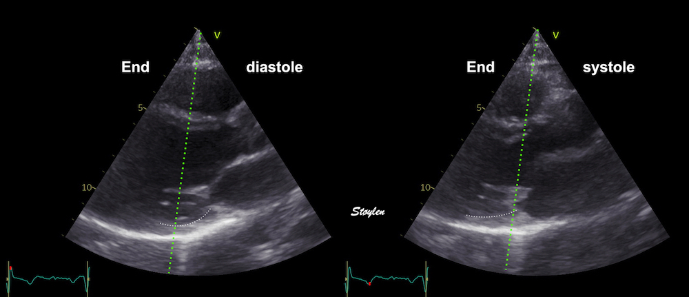
Immages from different parts of the heart cycle, showing that the line crosses different parts of the LV in end diastole and end systole. As the end systolic frame has moved the base of the heart further towards the apex, and the posterior wall thickens towards the mitral annulus, the motion induces an apperent over estimation of end systolic thickness, which will be reflected in the M-mode measurements:
The apparent higher thickening of the posterior LV, may thus be due to the increased thickness of the posterior wall moving into the M-mode line due to the longitudinal motion of the basal parts of the heart.
Pandian (36) by 2D measurements, found substantial heterogeneity of segmental thickening between segments, from WT 34 in septum to 57 in posterior wall, but not as systematic, and using short axis B-mode, may be vulnerable toi long axis basal motion as described for B-mode-
Comparing with longitudinal deformation of the two walls, we found in HUNT3 that MAPSE was about 14% higher in the posterior wall than the anteroseptum, but the posterior wall was also around 10% longer than the anteroseptum (156). Thus, the relative shortening (longitudinal wall strain) in HUNT 3 was 16.6% in the anteroseptum, vs 16.5% by segmental strain, and 14.7% vs 15.5% (relative difference 5%) by normalised MAPSE.
Thus, as longitudinal shortening and transverse thickening are interrelated as shown above, similar relative longitudinal shortenings between the walls, also indicates similar wall thickenings. Thus, the physiology weighs in favor of HUNT4 in this case, while the longitudinal and transmural deformation data in HUNT3 are somewhat inconsistent.
- Both studies, however, show very little decrease in endocardial FS with age.
- Both studies show decrease in relative wall thickening of both walls by age, which, at least in part is related to the age-dependent increase in wall thickness of both walls, found in both studies.
However, in HUNT4, With unchanged endocardial FS, and decreasing WT, it seems that this should add up to decrease in outer FS, as this is calculted from the basic measured, this must be an effect of increasing wall thickness with age, indicating that absolute wall thickening increased. his is in opposition to HUNT3, and what is true may still not be clear, although the decreasing outer diameter may bin HUNT3 may also be an effect of AV-plane motion as seen above..
Stroke volume can be derived from Doppler flow, as described above:
|
|
| |
Tracing the flow velocity curve by pulsed Doppler in LVOT through one heartbeat, gives the velocity time integral by the area under the curve. The LVOT diameter, can be measured in the B-mode. | The velocity time integral is the distance d, that somethin moving with the velocity of the traced curve moves, the stroke distance. The area A of the LVOT (assuming a circular cross section) is given by the measured LVOTdiameter. Thus, the volume of the cylinder given by d × A, equals the stroke volume. |
SV is also available by volumetry of the LV, both by 2D and 3D methods:
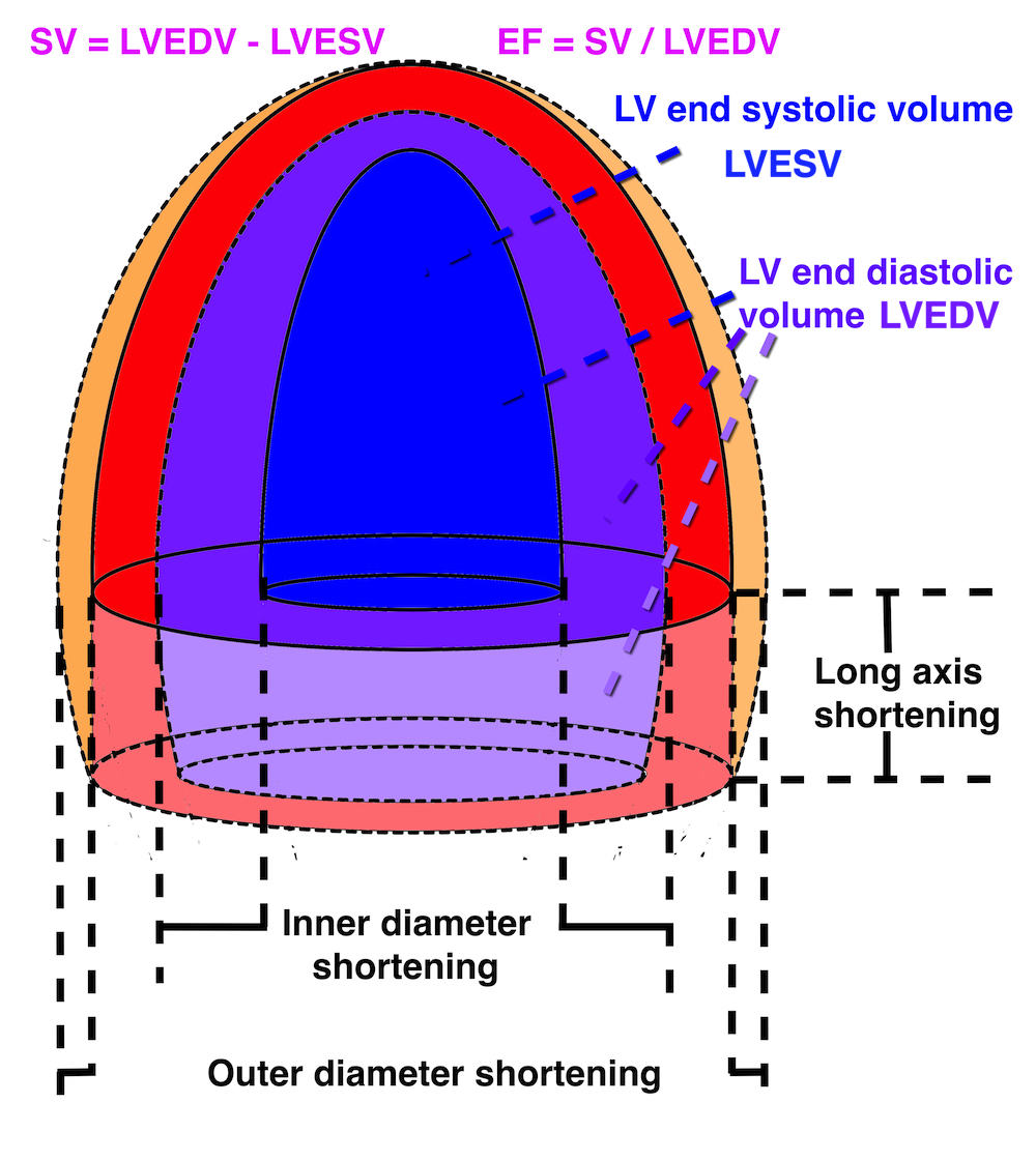
Simplified ellipsoid diagram of the LV, showing the principal relation of systolic and diastolic volumes as well as the relation to the dimension changes.

3D echo with LV volume curve. The volumes are all internal. Mark that the ejection curve is sigmoid, as the blood has inertia, the acceleration of the blood after AVO will take a certain time, and thus the maximum rate of volume decrease (=maximum flow rate) is delayed after AVO.
The delay after AVO follows necessarily after physics, instantaneous acceleration to peak flow is contrafectual, but is evident from LVOT Doppler, and has also been documented by volumetry (265, 266).
With a completely incompressible myocardium, the stroke volume would equal the reduction in outer volume, without taking cavity and wall thicknesses into consideration. As the incompressible myocardial volume remains constant, the outer volume reduction must equal cavity volume reduction as shown below.

The left figure shows the cavity volume reduction, being the function of longitudinal and endocardial transverse diameter shortening. But the right figure shows that the total LV outer volume is the sum of cavity and myocardial volume. Given a minimally incompressible myocardium, the reduction in total volume = reduction in cavity volume, while the myocardial volume is constant.
Total (outer) LV volume LVTV = Cavity volume + myocardial volume (MV).
Diastole: LVEDV = LVEDTV - LVEDMV
Systole: LVESV = LVESTV - LVESMV
SV = LVEDV - LVESV = (LVEDTV - LVEDMV) - (LVESTV - LVESMV) = LVEDTV - LVEDMV - LVESTV + LVESMV
If the myocardium is nearly incompressible is LVEDMV ![]() LVESMV then SV
LVESMV then SV ![]() LVEDTV - LVESTV
LVEDTV - LVESTV
Stroke volume ![]() systolic outer LV volume decrease
systolic outer LV volume decrease
While SV may be the most important result of cardiac pumping, it confers little information about the state of the heart itself. In a dilated heart, the stroke volume relative to the total cavity volume (LVEDV) can be reduced, but the absolute stroke volume may be maintained. Although the dilated LV may have an increased afteroad, according to the law of Laplace:
![]()
having a larger radius and thinner wall, the ejected volume in terms of the total volume is lower.
Ejection fraction is SV normalised for LVEDV: EF = SV / LVEDV. It is important to realise that Reduced EF, due to chronic dilation, is not related to the Frank Starling effect due to increased preload. In chronic dilation, the EF is a measure of reduced performance, while both dilated and normal ventricles which dilates as response to increased LVEDP, will show increased SV. However, EF will decrease in response to both acute and chronic increase in afterload.
Stroke volume and EF are thus preload dependent, contractility dependent, afterload dependent.
Thus, the ejection fraction is a measure of the relative performance of the LV, in dilated ventricles:
![]()
A dilated ventricle can maintain stroke volume, but it is reduced in terms of the left ventricle volume, and may have a severely reduced contractility, and by normalising the SV for EDV, one comes closer to a relative systolic perfomance. In assessing EF, however, it should be emphasized, however, that EF is not a direct measure of myocardial function, as it measures the cavity, not the myocardial deformation. At best, it could be characterised as an indirect measure.
|
|
Normal ventricle with normal EF | Dilated ventricle with increased LV volume, and sverely reduced EF. |
Ejection fraction is still the most widely used measure of systolic left ventricular function today. This is mainly due to the vast amount of prognostic information from earlier studies, and the prognostic interventions that are geared to a cut off point in EF, basically because inclusion usually was based on dilated conditions.
When EF is evaluated prognostically in an unselected population, however, when patients without dilation is included, it has been shown to be a poor prognosticator even in heart failure (136). This shows that there are shortcomings in the use of EF as a marker of cardiac performance. EF is not a direct measure of myocardial function, as it measures the cavity, not the myocardial deformation. At best, it could be characterised as an indirect measure, and this is the reason for this shortcoming, as will be explained below.
Applying the ellipsoid model to the HUNT3 data, gave the following values:
Age | LVEDV(ml) | SV(ml) | EF(%) | Myocardial volume d (ml) |
Women | ||||
<40 | 111.6(21.6) | 76.3(16.4) | 68(6) | 87.0 (19) |
40-60 | 106.9(21.7) | 72.7(17.0) | 68(6) | 92.8 (19.6) |
>60 | 97.9(19.7) | 65.4(16.9) | 66(9) | 95.6 (18.9) |
Total | 106.8(21.8) | 72.6(17.3) | 68(6) | 91.4 (19.6) |
Men | ||||
<40 | 144.8(30.5) | 96.1(22.9) | 66(8) | 125.3 (23.6) |
40-60 | 138.1(31.1) | 92.2(23.8) | 67(8) | 129.7 (25.3) |
>60 | 126.3(33.7) | 84.1(25.7) | 66(8) | 128.2 (26.8) |
Total | 136.6(32.2) | 91.0(24.4) | 67(8) | 128.4 (25.3) |
All | 121.1(31.1) | 81.4(22.9) | 67(8) | 101.4 (27.9) |
LV volumes in HUNT4
Volumes in HUNT 4 are 2D measurement derived, values given are taken from (249).
Comparing with the values from HUNT4 (249), which were measured in 2D, the values according to age and sex can be found in the original publication.:
Age (years) | LVEDV(ml) | SV(ml) | EF(%) |
Women | |||
20 - 39 | 114 (26) | 68 | 60 |
40 - 59 | 102 (19) | 62 | 61 |
60 - 79 | 84 (19) | 51 | 60 |
> 79 | 67 (7) | 41 | 62 |
All | 94 | 57 | 61 |
Men | |||
20 - 39 | 145 (28) | 84 | 58 |
40 - 59 | 136 (29) | 81 | 60 |
60 - 79 | 119 (27) | 71 | 60 |
> 79 | 104 (18) | 62 | 59 |
All | 128 | 76 | 59 |
Total | 109 | 66 | 60 |
SV is calculated from EDV and ESV, corrected for the numbers in each age class before averaging.
Compared to the ellipsoid model from M-mode derived values, both volume, SV and EF is lower, but the relation to age, with declining values in increasing age are the same. This of course follows from the simultaneous age dependent decrease in both LVIDd and LVILd by age in both studies. Myocardial volume is not calculated in HUNT4.
Finally, both studies show concomitant decrease in LVEDV and SV by age, which will maintain EF without any kind of cross sectional increase in contraction.
The NORRE study shows even lower EDV and SV (calculated from end systolic and end diastolic volumes given in the paper), but EF intermediate between HUNT 3 and 4. This study also shows that LVEDV decrease with age, while EF is stable. This, of course means that SV must decrease, (being SV = EDV × EF).
Heart size is obviously related to body size. In the HUNT3 study, LVEDV and SV were both related to body size (R = 0.70 and 0.50, respectively, both p<0.001) (65). EF, being the ratio of the two, is nearly not correlated with BSA at all and the weak correlation is negative (R = - 0.07, p < 0.01). Thus, EF is the only volumetric index that is BSA independent.
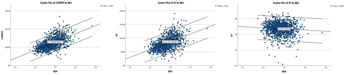
Diagram showing a strong correlation of both EDV and SV with body size, while there is only a very weak correlation of EF (being the ratio between the two) and body size.
As the base of the heart moves towards the apex, and the apex is stationary, the LV shortening (in absolute units, e.g. cm), must equal the motion of the LV base, i.e. the Mitral Annular Plane Systolic Motion (MAPSE).
|
|
As the apex is stationary, as shown by the upper line, the total systolic LV shortening is equal to the mitral annulus systolic motion towards the apex. | Mitral annulus motion can be assessed by the longitudinal M-mode through the mitral ring, and the total systolic mitral displacement - Mitral Annular Plane Systolic Excursion - MAPSE, equals LV systolic shortening. |
Global MAPSE is the mean of MAPSE measured in the septal and lateral point, or the mean of septal, anterior, inferior and lateral points or from all 6 walls.
MAPSE varies between sites in the LV (156, 221, 222):
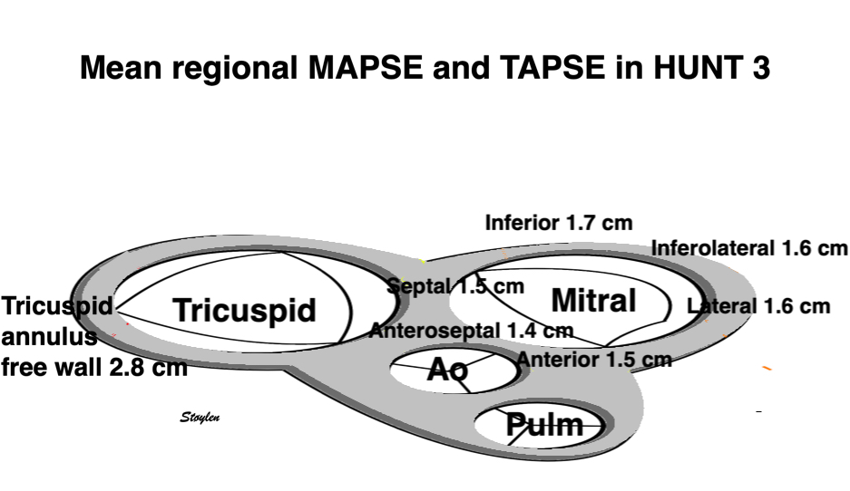
Mean AV-plane systolic displacement at different sites, showing the variability in the Mitral annulus, and TAPSE in the tricuspid annulius which is higher than any site in the mitral annulus.
We compared MAPSE from mean of 2 (septum and lateral wall), 4 (septum, lateral, anterior and inferior walls) and 6 (septum, lateral, anterior and inferior, ateroseptal and inferolateral walls).
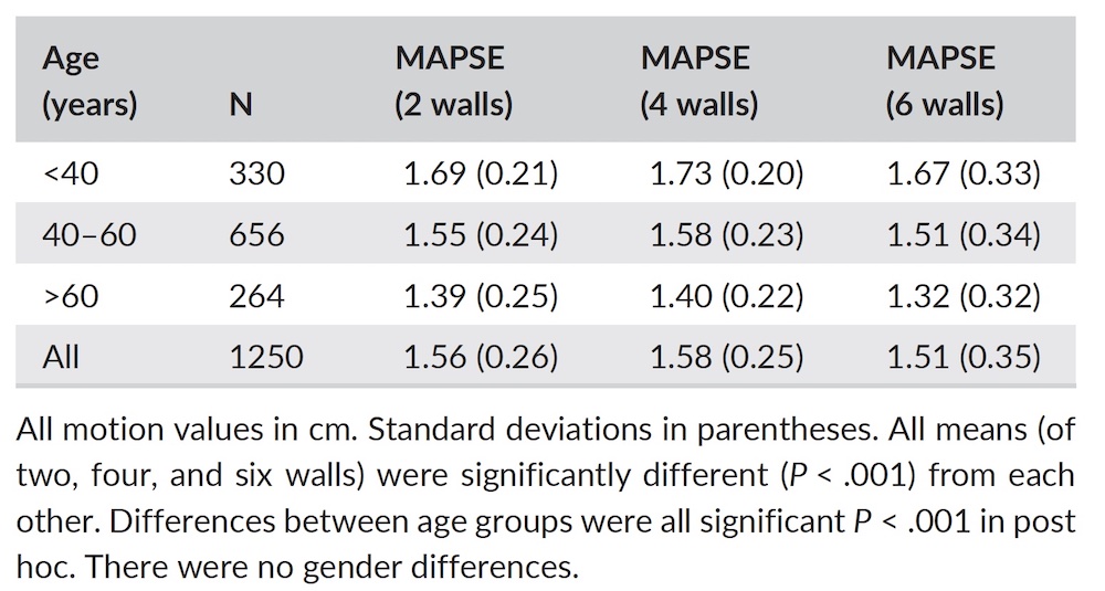
However, even if significant in a large study, differences between two, four and six walls were less than 1 mm, which is the limit for measurements in a simgle measure, so the averages were in practice identical. As we found less than 1 mm difference in MAPSE between the averages of 2, 4 and 6 walls in HUNT3, it seems that the number of planes are not of consequence for the mean values.
Age | N | MAPSE 4 walls | SEM | 95% CI |
Women | ||||
< 40 | 208 | 1.73 (0.20) | 0.013 | 1.704 - 1.756 |
40 - 60 | 336 | 1.58 (0.23) | 0.013 | 1.554 - 1.606 |
> 60 | 119 | 1.33 (0.22) | 0.020 | 1.29 - 1.37 |
All | 663 | 1.58 (0.26) | ||
Men | ||||
< 40 | 126 | 1.72 (0.22) | 0.020 | 1.69 - 1.76 |
40 - 60 | 327 | 1.58 (0.22) | 0.012 | 1.556 - 1604 |
> 60 | 150 | 1.45 (0.21) | 0.017 | 1.416 - 1.484 |
All | 603 | 1.58 (0.24) | ||
Total | 1266 | 1.58 (0.25) | ||
Relative SD (%) | 16 | |||
MAPSE is given with the mean for each age and sex group, the SEM is calculated, and the 95% CI for each group will then be mean ± 2 SEM.
Global strain is LV shortening normalised for LV length or wall length as explained here. The table shows global strain as MAPSE normalised for mean wall length (MAPSEn) and GLS by segmental strain, which is another linear method. Normalised MAPSE was done by normalising for wall length (or the straight line approximation of that). This means a skewed line slightly longer than the mid cavity straight line as discussed here. Using an ellipsoid model of the LV, calculated mean LV mid cavity length was 92.4 mm external, and 88.8 mm internal length. Mean MAPSE was 15.8 mm, which would result in a relative LV shortening (as opposed to wall shortening) of 17.1% using the external diameter, and 17.9% using internal diameter.
|
|
|
Normal distribution of MAPSE; skewness 0.003 | minimal positive correlation with BSA (R= 0.12, p<0.001) | negative correlation with age (R = - 0.50, p < 0.001) |
SV and EF are calculated from the ellipsoid LV model. SV, MAPSE, normalised MAPSE and GLS as well as TAPSE all declined by age. EF did not, as explained below, because of the concomitant decrease in LVEDV and SV, VTI did not for the same reason as peak LVOT flow velocity: As SV is a function of LVOT velocityintegral and LVOT area, this indicates that LVOT area possibly declines with age.
In the HUNT3 study, MAPSE was normally distributed, weakly correlated with body size, but in linear regression, sex differences was not significant. MAPSE was somewhat more strongly negatively correlated with age (18). In HUNT 4, Ventricular lengths and GLS were likewise normally distributed. Relation between relative shortening and GLS by speckle tracking, is discussed elsewhere.
Comparing with the values from HUNT4 (245, 249), which were measured in 2D the values according to age and sex can be found in the original publications. The LV lsystolic and diastolic lengths are presumably from volumetry, and thus are the internal lengths. SV is calculated from the difference in 2D systolic and diastolic volumes, EF both as given in (249) and calculated from LVEDV and SV. Measurements corrected for the numbers in each age class before averaging. Systolic and relative shortening are calculated from the basic length measurements, and likewise corrected for numbers. GLS are values from speckle tracking measurements in (245).
Volumetry by Simpson's method. It also gives internal LV lengths, which vcan be used for LV shortening calculations.
Age (years) | N | LVILd-4ch (cm) | SEM | LVILs4ch (cm) | SEM | Syst shortening-4ch | estimated SEM | 95% CI |
Women | ||||||||
20 - 39 | 64 | 8.5 (0.6) | 0.075 | 7.2 (0.5) | 0.063 | 1.3 | 0.138 | 1.024 - 1.576 |
40 - 59 | 357 | 8.3 (0.6) | 0.032 | 7.1(0.5) | 0.026 | 1.2 | 0.058 | 1.084 - 1.316 |
60 - 79 | 355 | 7.9 (0.6) | 0.032 | 6.8 (0.5) | 0.027 | 1.1 | 0.059 | 0.982 - 1.218 |
> 79 | 12 | 7.1 (0.5) | 6.4(0.4) | 0.7 | ||||
All | 8.1 | 8.2 | ||||||
Men | ||||||||
20 - 39 | 49 | 9.7 (0.6) | 0.086 | 8.1(0.5) | 0.071 | 1.6 | 0.157 | 1.286 - 1.914 |
40 - 59 | 284 | 9.2 (0.6) | 0.036 | 7.9 (0.5) | 0.030 | 1.3 | 0.066 | 1.168 - 1.432 |
60 - 79 | 279 | 8.9 (0.6) | 0.036 | 7.7 (0.5) | 0.030 | 1.2 | 0.066 | 1-068 - 1.332 |
> 79 | 12 | 8.5 (0.5) | 7.2 (0.5) | 1.3 | ||||
All | 9.1 | 9.2 | ||||||
Total | 8.5 | 8.6 | ||||||
SEM is calculated from the numbers in each age group, and the SD of the diastolic and systolic lengths, given in the paper. SEM of LV shortening (difference between lengths) is then conservatively assumed to be the sum of the SEM for each length, and the 95% CI is mean ± 2SEM. Comparing with the MAPSE values of HUNT3 in the table above, we see that the 95% CI are non-overlapping, except for the youngest male group, which has a rather wide CI due to the small size.
In general, we must conclude that the two studies show different values for almost all age groups (and thus, the difference is not due to the mean age difference of the two cohorts.
It is reasonable to assume that this is due to the difference in the methods used.
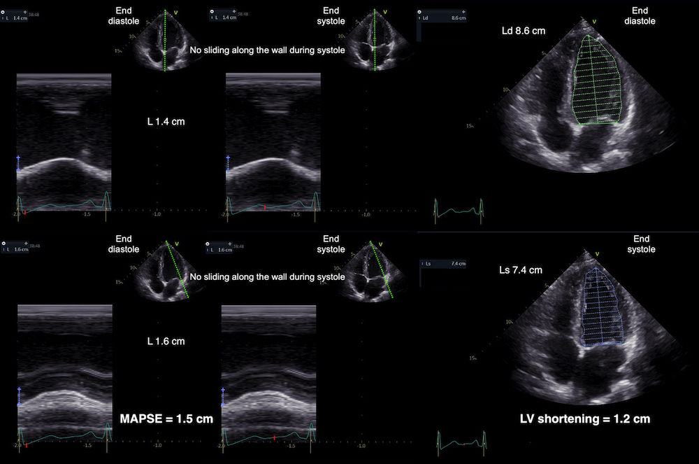
M-mode MAPSE and LV shortening by 2D from the same loop. The two methods give different values as discussed above. We also see that in this case, there is no M-mode artefact of the cursor sliding along the wall, ist is simply that while M-mode reflects external wall shortening, the internal shortening is less.
Thus the two methods are in no way interchangeable. Still, HUNT 4 confirms the decreasing absolute and relative LV shortening with increasing age found in HUNT3, as well as equal absolute, but lower relative shortening in men vs women..
LV shortening was calculated from diastolic and systolic LV lengths given in the paper and supplementary, which are exports from the endocardial traces from volumetry. As we see, both in HUNT 3 and 4, there is little difference in measuring LV shortening in 4-chamber alone or in mean of two planes (4 walls), but the findings of the two studies differ considerably.
The absolute and relative shortening by 2D, are thus less than the M-mode derived values of HUNT 3. This bias points to one or more systematic deviations in the methods.
Using caliper measurements of six points of the Mitral annulus on MR, Ochs et al (222) found AV-plane motion of 15 mm in 209 healthy subjects, in line with HUNT3. Sepulveda-Martinez et al, (251) in a direct comparison between Echocardiography M-mode and caliper based MR measurement in 111healthy subjects found a mean MAPSE of 17 mm, (in a younger cohort), and a bias of only 1 mm between the two methods. Thus, it seems that M-mode of the mitral plane is the most reliable, and that the HUNT3 describes the absolute LV shortening closer.
MR studies in gereal measures outer contour shortening (66).
The main reason is that the internal shortening is less that the external shortening, due to the dome shape of the LV. The mitral ring is a stiff structure, there is no Torsion during systole, and thus the ring motion follows the outer contour (wall) shorteni ng), despite being measured in the cavity.
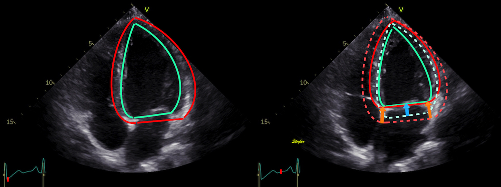
Internal (blue arrows) and external (orange arrows) LV shortening, showing that the external shortening is larger than the internal, due to the dome shape of the LV basis.. The M mode conforms with the external wall shortening, (even when measured internally, as the mitral ring is a rigid structure, and there is no torsion of the ring during systole.
Age (years) | SV (ml) | EF (%) | LVOT VTI (cm) | MAPSE (4 walls cm) | MAPSEn (4 walls %) | Segmental GLS (%) | TAPSE (cm) |
Women | |||||||
< 40 | 76.3 (16.7) | 68 (6) | 20.8 (3.5) | 1.73 (0.20) | 18.1 (2.0) | 17.9 (2.1) | 2.9 (0.5) |
40 - 60 | 72.7 (17.0) | 68 (7) | 21.6 (3.4) | 1.58 (0.23) | 17.0 (2.2) | 17.6 (2.1) | 2.7 (0.5) |
> 60 | 65.4 (16.9) | 66 (9) | 21.7 (3.7) | 1.33 (0.22) | 14.8 (2.1) | 15.9 (2.4) | 2.5 (0.56) |
All | 72.6 (17.3) | 68 (8) | 21.4 (3.5) | 1.58 (0.26) | 17.0 (2.4) | 17.4 (2.3) | 2.8 (0.5) |
Men | |||||||
< 40 | 96.1 (22.9) | 66 (8) | 20.0 (3.3) | 1.72 (0.22) | 16.5 (2.0) | 16.8 (2.0) | 3.0 (0.6) |
40 - 60 | 92.2 (23.8) | 67 (8) | 20.4 (3.6) | 1.58 (0.22) | 15.4 (1.9) | 15.8 (2.0) | 2.9 (0.6) |
> 60 | 84.1 (25.7) | 66 (9) | 20.3 (3.7) | 1.45 (0.21) | 14.9 (1.9) | 15.4 (2.4) | 2.8 (0.6) |
All | 91.0 (24.4) | 67 (8) | 20.3 (3.6) | 1.58 (0.24) | 15.5 (2.0) | 15.9 (2.3) | 2.9 (0.6) |
Total | 81.4 (22.9) | 67 (8) | 20.8 (3.6) | 1.58 (0.25) | 16.3 (2.4) | 16.7 (2.4) | 2.8 (0.5) |
Relative SD (%) | NA | NA | NA | 16 | 14 | 24 | NA |
Global strain is LV shortening normalised for LV length or wall length as explained here. The table shows global strain as MAPSE normalised for mean wall length (MAPSEn) and GLS by segmental strain, which is another linear method. Normalised MAPSE was done by normalising for wall length (or the straight line approximation of that). This means a skewed line slightly longer than the mid cavity straight line as discussed here. Using an ellipsoid model of the LV, calculated mean LV mid cavity length was 92.4 mm external, and 88.8 mm internal length. Mean MAPSE was 15.8 mm, which would result in a relative LV shortening (as opposed to wall shortening) of 17.1% using the external diameter, and 17.9% using internal diameter.
Age (Years) | SV(ml) | EF (measured %) | EF (calc %) | Syst. shortening (cm) 4-ch | Syst. shortening (cm) 2-ch | Mean shortening (cm) | Relative shortening (%) |
Women | |||||||
20 - 39 | 68 | 60 (4) | 60 | 1.3 | 1.3 | 1.3 | 15.2 |
40 - 59 | 62 | 61 (5) | 61 | 1.2 | 1.2 | 1.2 | 14.4 |
60 - 79 | 51 | 60 (5) | 61 | 1.1 | 1.1 | 1.1 | 13.9 |
> 79 | 41 | 62 (3) | 57 | 0.7 | 0.9 | 0.8 | 11.1 |
All | 57 | 60 | 61 | 1.2 | 1.2 | 1.2 | 14.2 |
Men | |||||||
20 - 39 | 84 | 58 (6) | 60 | 1.6 | 1.4 | 1.5 | 15.5 |
40 - 59 | 81 | 60 (5) | 60 | 1.3 | 1.4 | 1.4 | 14.5 |
60 - 79 | 71 | 60 (5) | 60 | 1.2 | 1.1 | 1.2 | 12.9 |
> 79 | 62 | 59 (5) | 60 | 1.3 | 0.9 | 1.1 | 13.0 |
All | 76 | 59 | 60 | 1.3 | 1.3 | 1.3 | 13.8 |
Total | 66 | 60 | 60 | 1.2 | 1.2 | 1.2 | 14.0 |
Mean values for each group are taken from (249) for lengths, and corrected for the numbers in each age class before averaging. Absolute and relative shortening are calculated from the basic measurements, and likewise corrected for numbers.
In HUNT3, the mean left ventricular internal length was calculated from wall lengths to 88 mm. In HUNT4, the internal LV length was 85 mm.
GLS is by speckle tracking, from (245), which is the same population (for comparison with absolute and relative shortening, GLS is given by numerical values):
<40 years | 40 - 49 years | 50 - 59 years | 60 - 69 years | > 69 years | All |
Women | |||||
21.3 (1.8) | 21.0 (2.2) | 20.5 (1.8) | 19.7 (2.0) | 19.0 (2.0) | 20.2 (2.0) |
Men | |||||
19.8 (1.9) | 20.1 (1.8) | 19.5 (1.8) | 18.9 (1.9) | 18.5 (2.1) | 19.3 (2.0) |
Total: 19.8 (2.1) | |||||
TAPSE was likewise normally distributed, and correlated negatively with age, positively with BSA, small gender differences were not significant in linear regression with BSA (103).
Both TAPSE and S'RV correlated modestly with BSA, and there was a sex difference, but this was simply due to BSA difference, as shown by linear regression.

The eggshell model of the heart would predict that the stroke volume would be solely the function of long axis shortening (12 - 14), at least with an incompressible myocardium. As discussed in the basics section, however, there is an outer diameter decrease as well (62, 63, 65), contributing to stroke volume. This can be seen here:

A>s seen here, the main deformation of the ventricles, is in the longtitudinal direction by AV-plane motion. Most transverse chamber reduction,m is due to wall thickening, which again is a function of shortening. But there is also an outer diameter reduction due to true circumferential fibre shortening, as discussed here, and this outer diameter reduction can be seen here.
With a completely incompressible myocardium, the stroke volume would equal the reduction in outer volume, without taking cavity and wall thicknesses into consideration. As the incompressible myocardial volume remains constant, the outer volume reduction must equal cavity volume reduction as shown below.
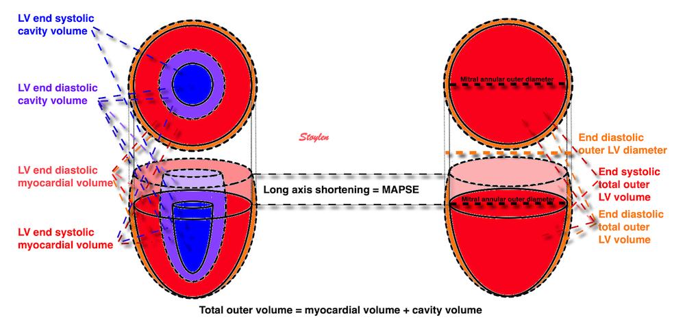
The left figure shows the cavity volume reduction, being the function of longitudinal and endocardial transverse diameter shortening. But the right figure shows that the total LV outer volume is the sum of cavity and myocardial volume. Given a minimally incompressible myocardium, the reduction in total volume = reduction in cavity volume, while the myocardial volume is constant.
Total (outer) LV volume LVTV = Cavity volume + myocardial volume (MV).
Diastole: LVEDV = LVEDTV - LVEDMV
Systole: LVESV = LVESTV - LVESMV
SV = LVEDV - LVESV = (LVEDTV - LVEDMV) - (LVESTV - LVESMV) = LVEDTV - LVEDMV - LVESTV + LVESMV
If the myocardium is nearly incompressible is LVEDMV ![]() LVESMV then SV
LVESMV then SV ![]() LVEDTV - LVESTV
LVEDTV - LVESTV
Stroke volume ![]() systolic outer LV volume decrease
systolic outer LV volume decrease
Outer volume decrease has two components:
Longitudinal component = MAPSE × Mitral annular outer area = MAPSE × ![]() outer mitral annular diameter / 2
outer mitral annular diameter / 2
Transverse component which is SV - longitudinal component.
In the HUNT study we used a symmetric, ellipsoid model of the LV, In the HUNT3 ellipsoid LV model, (65), we measured MAPSE and outer ventricular diastolic and systolic diameter, and assumed the mitral annular diameter to be equal to LV outer systolic diameter as shown by the figure above. Thus we calculatedThe SV from the cavity volumes, MAPSE × mitral annular area, to derive the MAPSE part of the SV, considering the remaining decrease to be due to the ourer LV diameter decrease. We found that MAPSE contributed 74.2% of total SV. Circumferential shortening due to OUTER circ. (diameter) shortening, was 12.8%, and must make up the rest, 25.8% of SV.

Although all primary measurements were normally distributed, the volumes were not, indicating that there was a systematic error in the geometrical model. This is reasonable, as the assumption of the model was a symmetric ellipsoid, which is not the case in real life.
Direct measurement by MR have shown that the AV-plane contribution is closer to 60% for the LV, but ca 80% for the RV (66, 67,68), which probably is closer, although a study of LV filling found that systole contributed 70% to ventricular filling (9), which should be equal to the ejected volume unless there is concomitant atrial expansion also.
Relations of MAPSE to SV
Age | MAPSE (cm) | SV(ml) | MAPSE vol(ml) | EF(%) | MAPSE% of SV | Endocardial FS(%) | Outer FS (%) | Wall thickening (%) |
Women | ||||||||
<40 | 1.73(0.20) | 76.3(16.4) | 56.5(9.9) | 68(6) | 75.4(11.9) | 36.6(6.1) | 14.1(3.3) | 61.7 (20.2) |
40-60 | 1.58(0.23) | 72.7(17.0) | 53.3(11.7) | 68(6) | 74.9(13.5) | 36.5(6.9) | 13.2(4.2) | 57.9 (19.6) |
>60 | 1.33(0.26) | 65.4(16.9) | 45.2(10.1) | 66(9) | 72.0(21.9) | 36.0(9.1) | 12.1(4.2) | 54.5 (19.8) |
Total | 1.58(0.26) | 72.6(17.3) | 52.9(11.5) | 68(6) | 74.6(14.9) | 36.4(7.1) | 13.3(4.0) | 58.5 (19.9) |
Men | ||||||||
<40 | 1.72(0.22) | 96.1(22.9) | 70.1(14.9) | 66(8) | 74.9(14.2) | 35.5(6.9) | 12.6(3.7) | 56.4 (19.1) |
40-60 | 1.58(0.22) | 92.2(23.8) | 65.1(14.2) | 67(8) | 72.8(14.8) | 35.8(7.4) | 12.2(3.8) | 54.6 (19.7) |
>60 | 1.45(0.21) | 84.1(25.7) | 60.3(14.7) | 66(8) | 74.9(19.0) | 36.0(8.0) | 11.8(4.4) | 51.8 (16.4) |
Total | 1.58(0.24) | 91.0(24.4) | 64.9(14.7) | 67(8) | 73.8(15.8) | 35.8(7.5) | 12.2(3.9) | 54.2 (18.8) |
All | 1.58(0.24) | 81.4(22.9) | 61.5(13.0) | 67(8) | 75.2(12.8) | 36.1(7.3) | 12.8(4.0) | 56.5 (19.6) |
We have calculated LV shortening from LV systolic and diastolic lengths, corrected for the numbers in each age class before averaging. With the same assumptioon as in HUNT3, that mitral annular diameter is close to LV external systolic diameter (LVEDs = LVIDs + LVPWs + LVIVSs), and the part of SV being LV shortening × ![]() × (LVEDS/2)2.
× (LVEDS/2)2.
Age (Years) | SV(ml) | EF (measured %) | EF (calc %) | Mean shortening (cm) | LV shortening vol (ml) | LV shortening vol (%) |
Women | ||||||
20 - 39 | 68 | 60 (4) | 60 | 1.3 | 28 | 41 |
40 - 59 | 62 | 61 (5) | 61 | 1.2 | 26 | 43 |
60 - 79 | 51 | 60 (5) | 61 | 1.1 | 23 | 45 |
> 79 | 41 | 62 (3) | 57 | 0.8 | 15 | 37 |
All | 57 | 60 | 61 | 1.2 | 25 | 44 |
Men | ||||||
20 - 39 | 84 | 58 (6) | 60 | 1.5 | 38 | 45 |
40 - 59 | 81 | 60 (5) | 60 | 1.4 | 36 | 44 |
60 - 79 | 71 | 60 (5) | 60 | 1.2 | 29 | 40 |
> 79 | 62 | 59 (5) | 60 | 1.1 | 27 | 44 |
All | 76 | 59 | 60 | 1.3 | 33 | 44 |
Total | 66 | 60 | 60 | 1.2 | 29 | 44 |
Mean values for each group are taken from (249) for lengths, and corrected for the numbers in each age class before averaging. Absolute and relative shortening are calculated from the basic measurements, and likewise corrected for numbers.
The findings in HUNT 4 deviates from HUNT3 both in absolute and relative long axis shortening, but also in the LV shortening contribution - both absolute and relative - to SV (despite lower SV).
This is somewhat surprising, and as the M-mode derived values
M-mode vs MR
Absolute og relative SV i Carlsson
While MAPSE correlates only weakly with BSA (R = 0.12, p<0.001), The MAPSE contribution to SV in % does not correlate with BSA at all. Thus, the MAPSE % of SV, being constant across the BSA range, MAPSE contribution in ml correlates strongly with BSA (R = 0.55, mp< 0.001) (65).
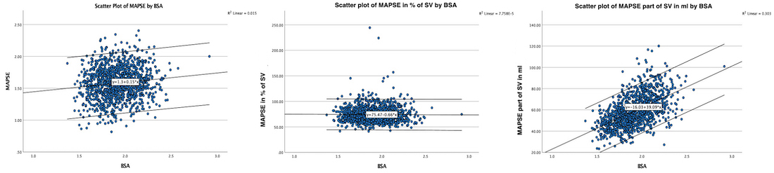
Diagrams showing the weak correlation of MAPSE with BSA, but also that the MAPSE percentage contribution to SV is BSA independent, which means, as SV is strongly BSA dependent, so is The MAPSE contribution in absolute volume.
The finding of unchanged EF and FS with increasing age, has been found numerous times (31 - 37), also in the HUNT 3 (65). It has been assumed that this was due to a "compensatory increase in short axis function". This argument was repeated by the finding of decreasing MAPSE with increasing age. However, this is not the case.
In the HUNT study half ellipsoid model of the LV based on linear measures (65), the MAPSE contribution to the SV would be external mitral annulus x MAPSE, while the transverse diameter shortening would contribute the rest. The aim of this study was primarily to study the age related changes in strains in relation to EF and stroke volume, as any systematic error might be assumed to be more or less constant across the study group. We found that EDV and SV declined with age. EF was unchanged by age, the mechanism for this was the concomitant decrease in EDV and SV, preserving the ratio.
MAPSE declined with age as shown previously (7, 18, 65), but not the MAPSE percentage of the SV, again due to the concomitant decrease of both measures.
Thus the preserved EF despite decrease in long axis function is NOT due to any compensatory increase in transverse function, all thre strains decline with age. The preserved EF is due to the simultaneous reduction in EDV, SV and MAPSE.
In the HUNT ellipsoid model, we looked at the changes in dimensions and volumes, SV, EF and FS in relation to ageing (65): The systematic error can be assumed to be more or less the same across age groups, and thus the findings in relation to ageing mif´ght be assumed to be valid.
In the HUNT study, we found in addition near unchanged LVIDD, unchanged FS and increased wall thickness, but with decreased wall thickening (relative).
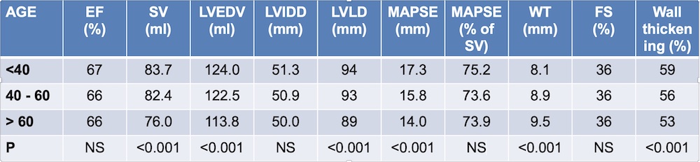
Thus, there is no "compensatory short axis increase as mechanism for maintained EF.
Methodologically, this shows that EF and FS are not sensitive for age related changes.
The long axis shortening and lengthening are thus related to annular displacement, and the displacement curve is closesly related to the absolute volume curve. The annular velocity is the first derivative of the displacement curve, just as the flow is the first derivative of volume.
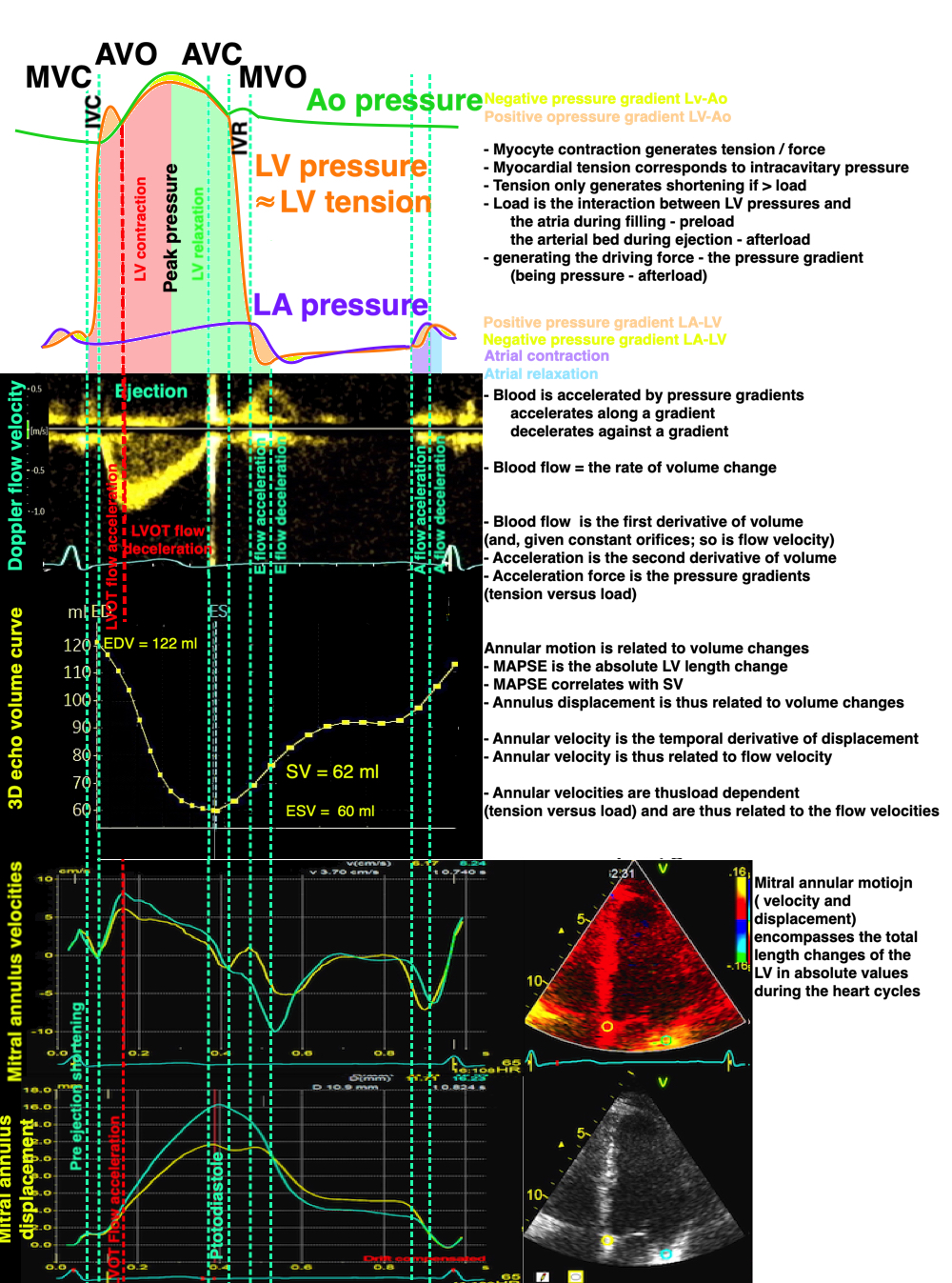
Relation of pressures, flow velocity, volumes, annular velocity and displacement. Length and velocity are both related to volume changes, and are the resultant of tension vs. load. Both E and e' are related to tension vs load, and e' is not the cause of early pressure changes.
|
|
Normal ventricle with normal EF | Dilated ventricle with increased LV volume, and sverely reduced EF. |
In dilated ventricles, the increasing LVEDV will cause the EF to decrease, despite normal SV. Thus, the EF is a more sensitive measure than SV. Likewise, the FS will be rediced as LVIDD increases in dilation.
Ejection fraction is still the most widely used measure of systolic left ventricular function today. This is mainly due to the vast amount of prognostic information from earlier studies, and the prognostic interventions that are geared to a cut off point in EF.
MAPSE will also be reduced in dilated heart failure:

When the left ventricle dilates, both the volume and diameter increases, and the stroke volume can be maintained by a smaller fraction (Ejection fraction) of the total (end diastolic) volume. As the stroke volume is proportional with the MAPSE x outer area, as discussed above, the SV also can be maintained with a lower MAPSE and a larger diameter, and there will be a near linear relation between reduction in EF and MAPSE.
The longitudinal shortening has been shown to be very closely related to ejection fraction when comparing different patients with normal or reduced left ventricular function (95, 133 - 136). The relation between MAPSE and EF has shown a correlation of 80 - 90%. However, the relation only holds in the spectrum from normal to dilated ventricles, when both are included. In a population of only normal ventricles, this correlation is not present, here MAPSE correlates with SV (137). Finally, there is no correlation of MAPSE with EF in hypertrophic ventricles (138).
While EF is a prognosticator in heart failure with dilatation, the same is not the case in a general heart failure population (131). This is due to the presence of heart failure with preserved ejection fraction HFpEF.
Patient with amyoloidosis and heart failure:
|
|
|
PSLAX | PSSAX | A4CH |
Evident is the thick wall and the small cavity. Systolic function is not normal, as the small cavity is unable to generate a normal SV, but as both LVEDV and SV are reduced, their ratio (EF) may be normal. MAPSE, however, will bve reduced also here.
MAPSE on the other hand, will be reduced, in line with the reduced SV, despite normal EF (139).
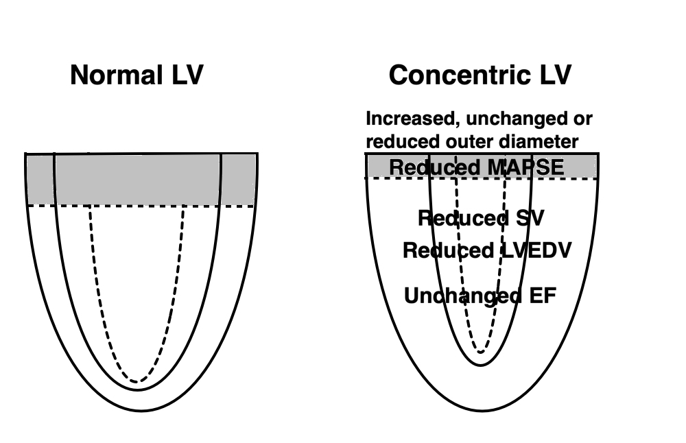
In concentric hypertrophy the LVEDV is reduced, and unable to generate the same SV. But as both LVEDV and SV are reduced, the EF may be preserved (HFpEF). The outer diameter may be increased, unchanged or reduced, depending on the pattern of wall thickness increase. Still the SV is proportional to the MAPSE x area, as discussed above, there will be a linear relation between the decrease in MAPSE and SV.
Concentric hypertrophy reduces the cavity volume, as well as the stroke volume, and the concomitant reduction of both can maintain the ratio between them. Thus, the EF or FS is a measure that actually only works with dilation of the ventricles and becomes erroneous in the cases of reduced EDV. EF is a geometrical concept, and only works in some geometries. MAPSE will decrease in relation to the reduction in SV.
The lack of understanding of the geometry of EF, has led to two misconceptions:
It is very common to hear that as longitudinal function decrease with age or hypertrophy or whatever, the short axis function shows compensatory increase. Especially if EF is preserved. This mis conception artises from the confusion between cavity and wall measures. In the HUNT study, LV internal diameter, and fractional diameter shortening did not change significantly) with increasing age, while wall thickness increased, and wall thickening (transmural strain) decreased (19, 7).
Age (years) | LVIDd (mm) | FS (%) | Wall thickness (mm) | Wall thickening (transmural strain %) |
< 40 | 51.3 | 36 | 8.1 | 59.1 |
40 - 60 | 50.9 | 36 | 8.9 | 56.3 |
> 60 | 50.0 | 36 | 9.5 | 53.0 |
The finding of unchanged LVIDD and FS has been confirmed before (32 - 37). Thus, there is no sign of increases cross sectional function in increasing age, even with preserved EF (65).
It has also been maintained as a mechanism for preserved EF in HFpEF, as longitudinal function is shown to be reduced. However, this is not found in direct studies of hypertrophy with HFpEF (80- 82).
The reason for the confusion is the different relations of cavity and wall measures to hypertrophy:
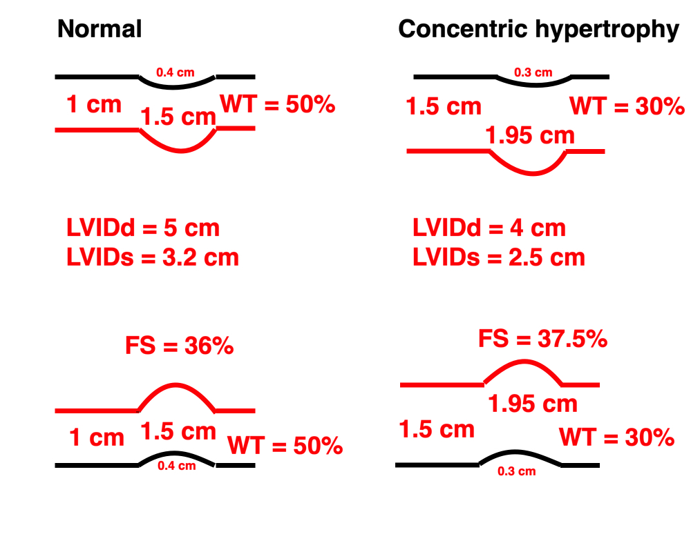
Schematic diagram of M-mode, illustrating the relation between cavity measures and wall measures of function. For simplicity, the ventricle is assumed to be symmetric. Left, a normal ventricle with wall thickness of 1 cm, systolic wall thickening of 50% and a systolic 11% outer diameter reduction. This gives a fractional shortening of 36%. Right a concentric hypertrophic ventricle with reduced myocardial function. The wall thickness is increased to 1.5 cm, outer diameter is the same, outer diameter shortening is reduced to 8.6%, wall thickening, while nearly the same in absolute measurement, is now only 30% relative. Fractional cavity diameter shortening, however, is slightly increased to 37.5%, but this is a function of the diastolic diameter reduction, nothing else. The true short axis function is the wall thickening, which is reduced.
So in this case, the short axis function is reduced, not increased, and the apparent increase in FS is in fact a decrease in both EDD, absolute shortening, and wall thicke4ning, preserving or increasing their ratio, analoguous with the volumes in EF.
The above example is an illustration, showing that in some instances, especially hypertrophy, the cavity measures do not measure the myocardial function, and the apparent "increased short axis function" is illusory, based on a misconception. An example illustrates this.
|
|
|
Patient with heart failure. EDV 100 ml, EF 55%, thus SV 55 ml. | Wall thickness 17 mm, EDD 40 mm. | FS 35%, however, wall thickening 28% |
Thus, in HFpEF, both cavity and LVIDD are reduced, while EF and FS are preserved.
|
|
MAPSE = 5 mm | S' = 3 mm |
The annular displacement has been shown to be more sensitive than EF in predicting events in heart failure (140, 141) and hypertension (142). Also, the MAPSE correlates better with BNP in heart failure, that the fractional shortening (143).
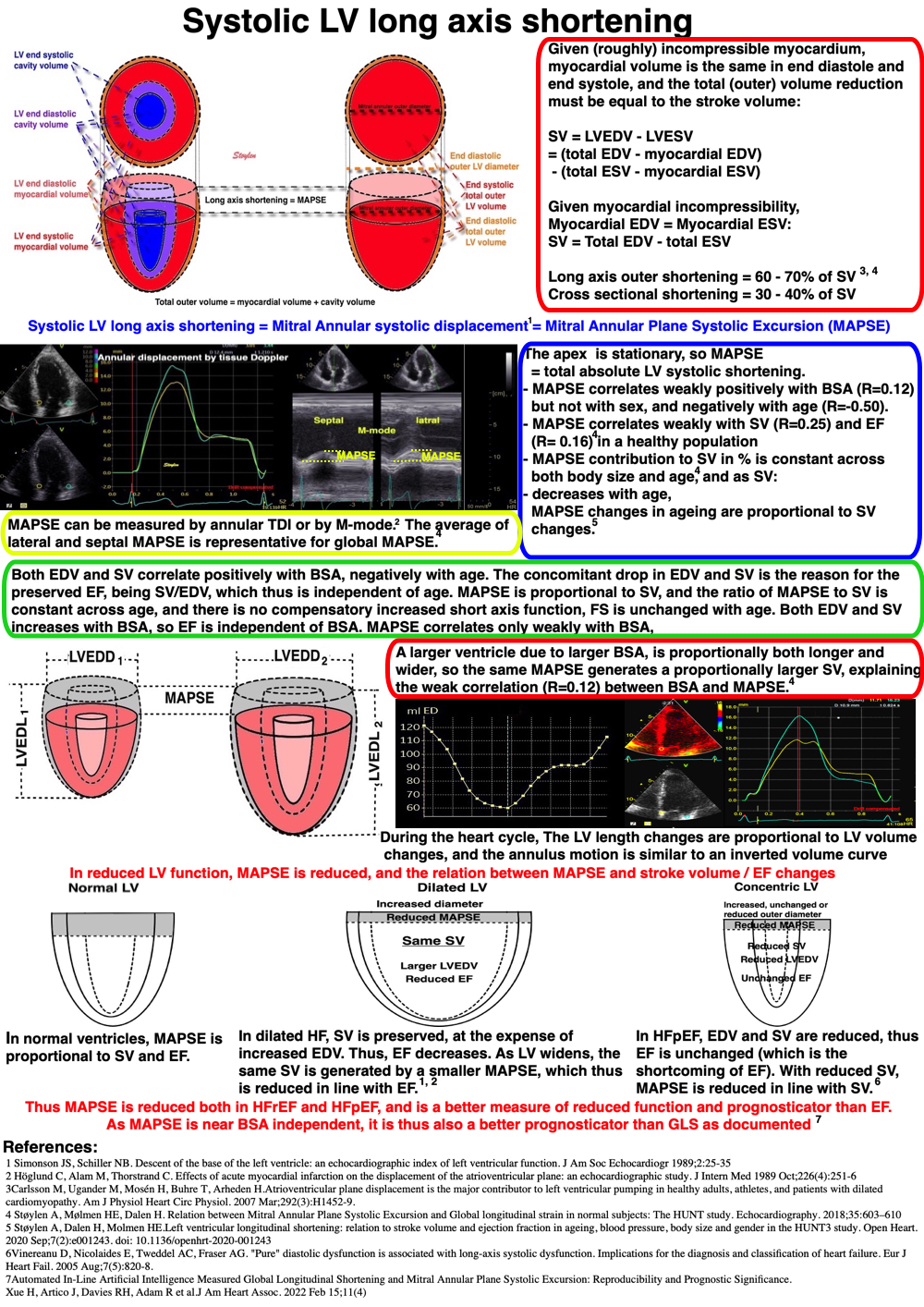
Looking at the systolic AV-plane displacement, the displacement varies intra individually with the site (156), in the LV highest laterally, both by M-mode (221) and by MR (222), but higher in the RV free wall than the LV lateral wall, (156) also found by others (223, 224). This is true also for S', as well as for wall lengths (16), so velocity and diasplacement varies concordantly (156). Looking at wall lengths, we have previously fond that in the LV the variation followed the same pattern (19).

Example of intra individual variability of LV wall lengths (measured as the straight line from the mitral annulus to the apex), annular plane displacement by M-mode, and S'. All are examplified by the septal and lateral measures, showing that both displacement and S' are highest in the RV free wall, lowest in the septum, higher again in the LV lateral wall than the septum. In the LV, the lateral wall is longer than the septum.
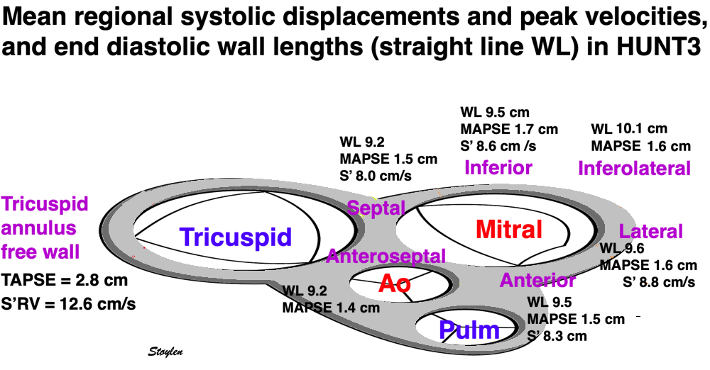
Mean AV-plane systolic displacement and velocities at different sites, showing that the highest displacement and velocity in the LV is in the lateral annulus, lowest in the septum, and the S' and TAPSE in the tricuspid annulius is higher than any site in the mitral annulus.
Looking at Mitral and tricuspid annular velocities (16), MAPSE/TAPSE (156) and LV strain rate and strain (17) per wall, the pattern is fairly consistent.
As all walls in the LV works at the same pressure (load), differences in wall shortening must reflect differences in contractility, i.e shortening vs load must be the same.
This, however, is not the same for the RV, where load is considerably lower, and the wall is longer.
Septal | Anteroseptal | Anterior | Lateral | Inferolateral (posterior) | Inferior | Relative, intraindividual variance (var / mean) | |
WL (cm) | 9.2 (1.7) | 9.2 (1.9) | 9.5 (1.8) | 9.6 (1.8) | 10.1 (2.1) | 9.5 (1.8) | 0.4 |
Displacement (MAPSE) (cm) | 1.5 (0.3) | 1.4 (0.4) | 1.5 (0.3) | 1.6 (0.3) | 1.6 (0.4) | 1.7 (0.3) | 0.03 |
MAPSE / WL (%) | 16.2 (2.8) | 14.7 (3.6) | 15.9 (2.8) | 16.3 (2.7) | 15.5 (3.6) | 17.1 (3.0) | 0.003* |
S' (cm/s) | 8,0 (1.2) | 8.3 (1.9) | 8.8 (1.8) | 8.6 (1.4) | 0.1 | ||
S' / WL (s-1) | 0.85 (0.13) | 0.85 (0.2) | 0.90 (0.19) | 0.88 (0.14) | 0.87 (0.14) | 0.01* |
Population means, and population standard deviations in parentheses. *p < 0.001 for difference of relative variance of normalised versus non normalised measures.
Normalising MAPSE and S' for wall length, reduced the relative intra individual variance by a factor of 90%, showing clearly that the systolic displacement and systolic displacement velocity were clearly related to wall lengths. As all walls of the LV works with similar afterload, this shows that contractility (i.e. shortening per length, is similar in all walls), related to the number of sarcomeres in series.
This is evident as also S' is related to wall length, i.e. the regional velocity / acceleration is a function of force.
Normalised MAPSE is a measure of strain (18), normalised S' a measure of strain rate (23).
Segmental strain and strain rate can also be seen to have far less variability than displacement and S', but we didn't react to this in the original studies (16, 17).
Thus, the LV motion is greatest in the lateral parts where the wall is longer, and shortening relative to wall length (wall strain) is more constant, consistent with a relatively uniform longitudinal sarcomere shortening in the LV.
Normal annular peak systolic velocities, strain rate and strain per wall in the HUNT study by tissue Doppler.
Anteroseptal | Anterior | (Antero-)lateral | Inferolateral | Inferior | (Infero-)septal | |
PwTDI S' (cm/s) | 8.3 (1.9) | 8.8 (1.8) | 8.6 (1.4) | 8.0 (1.2) | ||
cTDI S' (cm/s) | 6.5 (1.4) | 7.0 (1.8) | 6.9 (1.4) | 6.3 (1.2) | ||
SR (s-1) | -0.99 (0.27) | -1.02 (0.28) | -1.05 (0.28) | -1.07 (0.27) | -1.03 (0.26) | -1.01 (0.25) |
Strain (%) | -16.0 (4.1) | -16.8 (4.3) | -16.6 (4.1) | -16.5 (4.1) | -17.0 (4.0) | -16.8 (4.0) |
Values are mean values (SD in parentheses). Velocities are taken from the four points on the mitral annulus in four chamber and two chamber views, while deformation parameters are measured in 16 segments, and averaged per wall. The differences between walls are seen to be smaller in deformation parameters than in motion parameters, although still significant due to the large numbers.

Colour Doppler traces of velocity, displacement, strain and strain rate from the septal (yellow) and lateral (cyan) aspect of the four chamber view. motion traces are from the base,, deformation traces are from the whole wall as shown by the regions of interest (ROI). Systolic motion is positive, towards the probe. Systolic strain rate and strain is negative, as they represent shortening, and this is also evident from the definition of the velocity gradient / Strain rate. From this diagram, it is also evident that the velocities and displacements are higher in the lateral wall than the septum, while strain rate and strain are nearly equal. This is due to the fact that wall strain rate and strain basically are annular velocity and displacement normalised for wall length, and the lateral wall is longer than the septum.
The LV is often shown as a symmetric half-ellipsoid, but in reality, it is a skewed ellipsoid with the apex aligned with the centre of the AV - plane and the septum, which thusis shorter and straighter than the lateral wall.
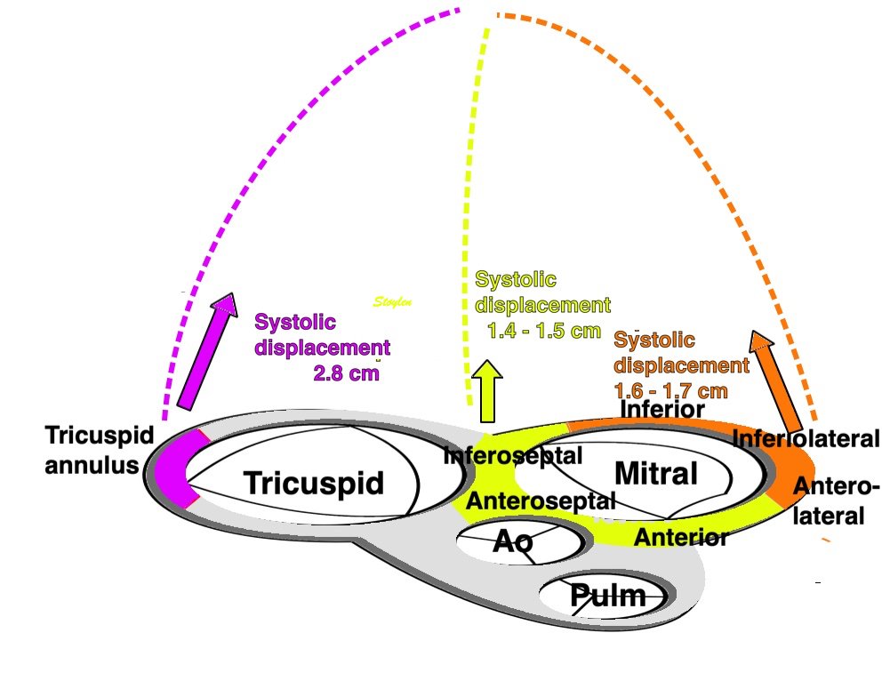
The relation of cardiac anatomy to regional AV-plane motion. The figure shows the longer walls in the lateral aspects, and shorter walls near the septum, and this relates to the position of the apex over the central part of the AV-plane. The central part of the AV-plane also is the site of the large arteries, which may anchor the AV-plane in the middle. The mean AV plane motion in the different sites are indicated, showing correspondence with WL in the LV.
The large arteries are anchored in the centre of the AV‐plane and must stretch during the systolic AV‐plane motion, so the differences in AV‐plane motion are related both to wall length and to the location of the large arteries, and hence, to the overall anatomy.
Shortening of the RV is greater than the LV, but RV wall is thinner and longer and works against a lower afterload, and hence tension, so the shortening relation to wall length it is not comparable with the LV. As RV motion is only measured in one wall, there are no other walls with similar load for comparison, and a direct comparison of shortening vs length between RV and LV is not relevant, but both interacts with the AV-plane.
Thus, the AV‐plane not only move towards the apex, but also bends into a U‐shape during systole, so not only the ventricular length, but also the width of the AV‐plane and the maximal width of the ventricles are reduced as well as tilts towards the left as shown below.
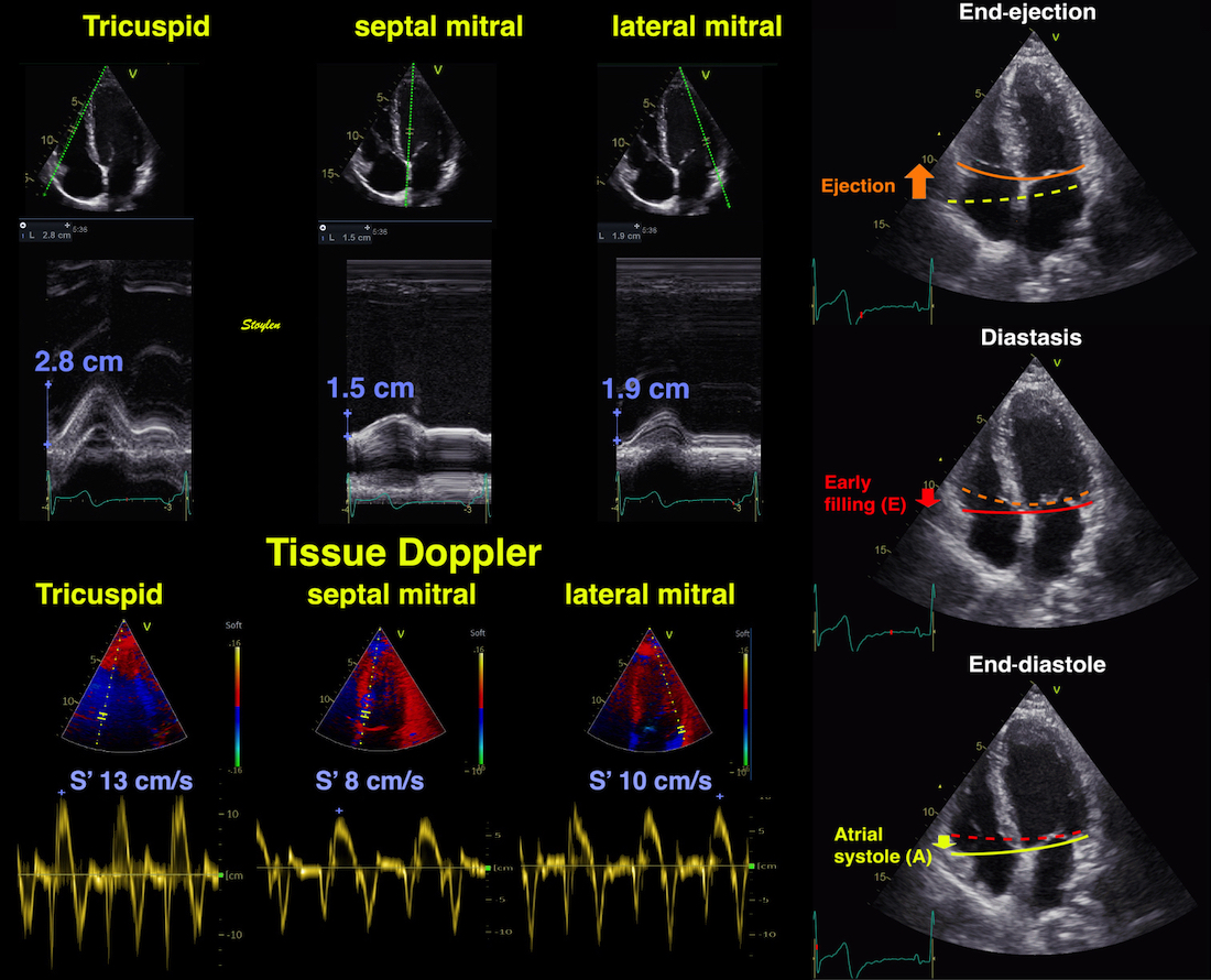
Example from a single subject. As seen both AV-plane systolic motion and AV-plane peak systolic velocity are highest in the rght lateral part, and lowest in the central part. This means that the differential motion will correspond to a systolic bending of the AV-plane, and a tilting towards the left.
What are the functional significance of the systolic AV-plane bending?
The systolic bending is evident also from the systolic velocities, but from this table it is also evident that most of the unbending happens in early diastole (highest e' in the RV, lowest in the septum), while the av-plane remains straighter, but with a tilting towards the right during atrial systole (highest in the RV, lowest in the left lateral)
Normal annular peak S', e' and a' per wall in the HUNT study by tissue Doppler.
Right ventricle | Anterior | septal | Inferior | lateral | |
PwTDI S' (cm/s) | 12.6 (2.1) | 8.3 (1.9) | 8.0 (1.2) | 8.6 (1.4) | 8.8 (1.8) |
PwTDI e' (cm/s) | 12.9 (3.2) | 11.6 (3.7) | 9.9 (2.9) | 11.2 (3.5) | 12.5 (3.7) |
PWTDI a' (cm/s) | 14.3 (3.8) | 9.4 (2.3) | 10.2 (2.2) | 11.0 (2.3) | 9.4 (2.4) |
|
|
|
In a modified eggshell model, there is also a reduction in outer transverse diameter, due to both outer ventricular diameter reduction and to AV-plane bending. The AV-plane apical motion is responsible for most of the ventricular systolic volume compression (red) and thus most of the the ejection volume, but in addition the volume is reduced by outer circumferential fibre contraction, and AV plane compression by bending, causing reduction in transverse diameter adding to the volume reduction (orange) and ejection. The atrial expansion, however, and thus the systolic venous inflow (S-wave), is mostly equal only to that caused by AV-plane motion. | During early filling there is recoil of the AV-plane, but only partly back to the end diastolic position, causing ventricularisation of part of the atrialised volume behind the compressed AV-plane (light red). This effect do not generate flow. The unbending of the AV-plane will cause an additional reduction of the atrial volume (violet), causing pressure rise (the V-wave), and atrioventricular early flow. | Atrial contraction will empty the auricles, giving an additional volume (light blue) that is injected into the ventricles, causing the final ventricular expansion back to the end diastolic position. This injection of blood causes pressure rise in atrium, |
Below is a clinical example corresponding to the diagrams above:
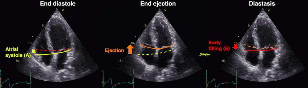
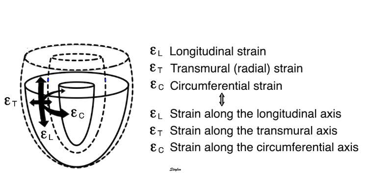
The three main coordinates of the heart: longitudinal, transmural and circumferential. This is the normal strain tensors, in this coordinate system, i.e. the coordinates of the deformation.
Global strain is basically left ventricular shortening normalised for end diastolic length. As discussed here, there is no universal standard, as the numerator depends on the method for tracking, and the denominator on what is chosen for reference length.
Inward tracking, is a property of feature tracking, and will result in apparent longitudinal shortening of the midwall and endocardium, even, hypothetically, without any ventricular shortening at all. This is due to the conical shape of the LV.
However, the common ground is that it is the left ventricular shortening, normalised in some way by LV end diastolic length. As MAPSE related to stroke volume, so did GLS.
It was shown early in experimental studies, that while peak strain rate was more closely related to contractility (ventricular elastance and inotropy) , end systolic strain and MAPSE was more closely related to SV and EF (127 - 130). The close relation of LV volume change and strain is shown below:
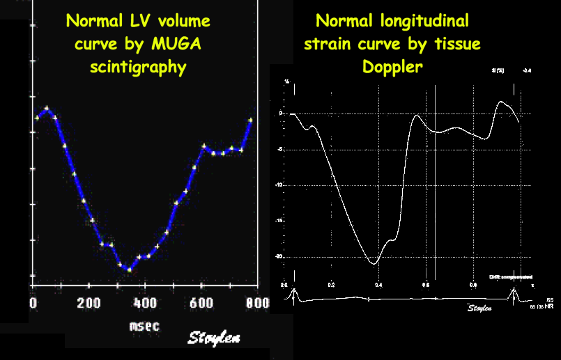
The picture shows a detailed LV volume curve from a healthy person by MUGA scintigraphy, the left a normal longitudinal strain curve. The similarity shows:
the volume changes of ejection and filling are closely related to the changes of the LV longitudinal dimension. However, as the left shows volume changes, while the right shows wall length changes, and as wall length changes vary between walls, the correspondence is not perfect.
In the HUNT3 study, using the geometrical model, Global MAPSE correlated woth normalised global MAPSE (R=0.86), GLS by segmental strain (R=0.40), S' (R=0.34), SV (R=0.25) and EF (R=0.16), all p<0.001). The two methods for GL correlated with each other (R=0.52), with S' (R=0.26 and 0.44, respectively), with EF (R=0.22 and 0.24), all p<=.001). However, GLS by either method do not correlate with SV (156). The possible explanation is the previous finding that SV is related to both LV length and diameter, which are interrelated, while global LV strain only normalizes for LV length, thus introducing a systematic error as described above. The SV in this comparison, however, is derived from a geometrical model (65), which in itself may include a systematic error, but the concordant results between the two strain methods, as well as the maintained relation of SV with MAPÅSE and S’, supports this finding.
Both segmental tissue Doppler derived GLS, normalised MAPSE and MAPSE itself, were normally distributed.

Normal distributions of MAPSE, MAPSEn, and GLS, with skewnesses of 0.003, -0.17 and 0.19, respectively.
It does seem intuitive that normalising MAPSE for length (ventricular or wall), should reduce the part of biological variability due to body size (heart size). In the HUNT study, however, we found that both segmental strain by tissue Doppler (17), as well as by the linear method (MAPSE normalised for wall length) (18), compared to non-normalised MAPSE with relative standard deviations were similar for all three methods.
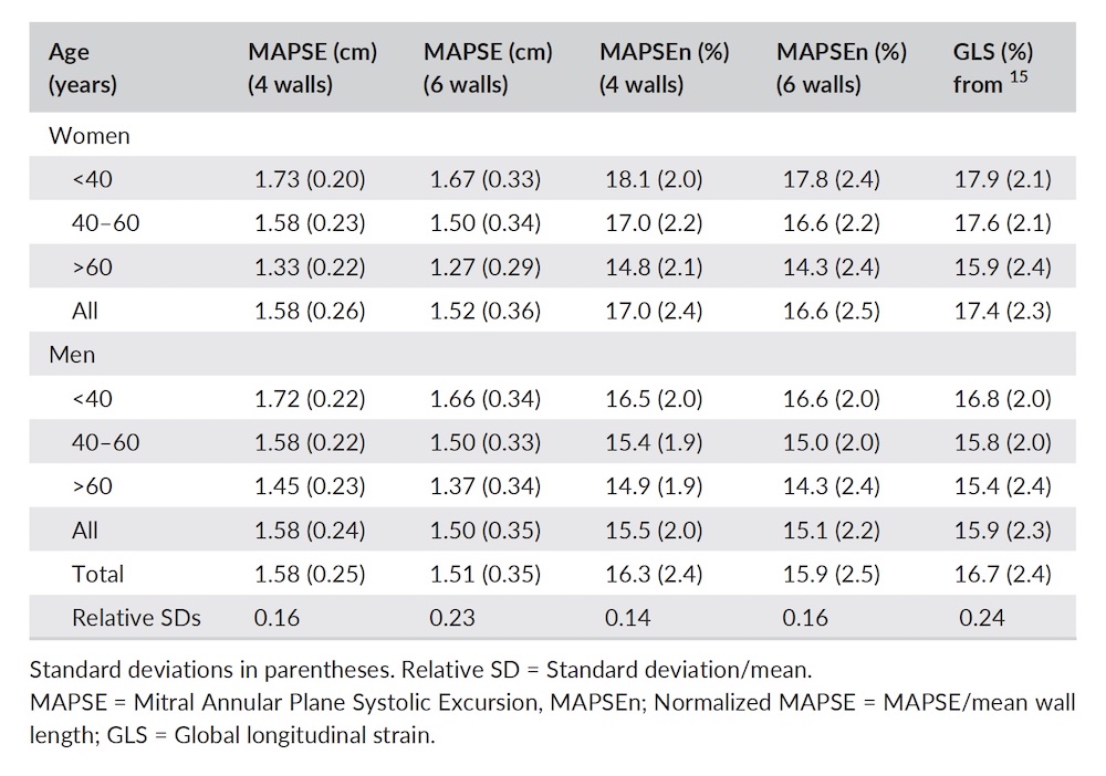
The finding that normalisation for LV length did not reduce biological variability, was perhaps a bit surprising, but is explainable as age is the source of the most variability (18)
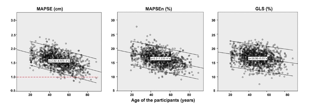
Age | MAPSE (cm) | MAPSE vol(ml) | LVEDV(ml) | SV(ml) | EF(%) | MAPSE% of SV | Endocardial FS(%) | Outer FS (%) | Myocardial volume d (ml) |
Women | |||||||||
<40 | 1.73(0.20) | 56.5(9.9) | 111.6(21.6) | 76.3(16.4) | 68(6) | 75.4(11.9) | 36.6(6.1) | 14.1(3.3) | 87.0 (19) |
40-60 | 1.58(0.23) | 53.3(11.7) | 106.9(21.7) | 72.7(17.0) | 68(6) | 74.9(13.5) | 36.5(6.9) | 13.2(4.2) | 92.8 (19.6) |
>60 | 1.33(0.26) | 45.2(10.1) | 97.9(19.7) | 65.4(16.9) | 66(9) | 72.0(21.9) | 36.0(9.1) | 12.1(4.2) | 95.6 (18.9) |
Total | 1.58(0.26) | 52.9(11.5) | 106.8(21.8) | 72.6(17.3) | 68(6) | 74.6(14.9) | 36.4(7.1) | 13.3(4.0) | 91.4 (19.6) |
Men | |||||||||
<40 | 1.72(0.22) | 70.1(14.9) | 144.8(30.5) | 96.1(22.9) | 66(8) | 74.9(14.2) | 35.5(6.9) | 12.6(3.7) | 125.3 (23.6) |
40-60 | 1.58(0.22) | 65.1(14.2) | 138.1(31.1) | 92.2(23.8) | 67(8) | 72.8(14.8) | 35.8(7.4) | 12.2(3.8) | 129.7 (25.3) |
>60 | 1.45(0.21) | 60.3(14.7) | 126.3(33.7) | 84.1(25.7) | 66(8) | 74.9(19.0) | 36.0(8.0) | 11.8(4.4) | 128.2 (26.8) |
Total | 1.58(0.24) | 64.9(14.7) | 136.6(32.2) | 91.0(24.4) | 67(8) | 73.8(15.8) | 35.8(7.5) | 12.2(3.9) | 128.4 (25.3) |
All | 1.58(0.24) | 61.5(13.0) | 121.1(31.1) | 81.4(22.9) | 67(8) | 75.2(12.8) | 36.1(7.3) | 12.8(4.0) | 101.4 (27.9) |
Basically, the findings of the functional measures were:
In this study, SV calculated from EDV-ESV in the ellipsoid model was 81.4ml, while Mitral area x MAPSE was 61.5 ml, = 74.2% of total SV. Circumferential shortening due to OUTER circ. (diameter) shortening, was 12.8%, and must make up the rest, 25.8% of SV.
Endocardial FS and EF did not decline with age, as has been shown many times before, (33, 34, 35, 250, 252, 253). But as internal FS is stable, and external FS decline with age, there is no compensatory increase in transverse (short axis/circumferential) function to maintain EF, it's simply the simultaneous decline in LVEDV and SV, that maintains their ratio. And this is not due to decrease in short axis internal diameter, but to a decrease in length (19).
MAPSE declined with age as described before (18). But just as for EF, the simultaneous decline in MAPSE and SV, maintains their ration, so the percentage of the SV due to MAPSE doesn't decline, and thus there is no need for any increase in transverse function. In fact, there is a decrease in midwall and outer FS, so there is a decline in transverse function with age (7).
In addition, MAPSE was independently related to DBP (Age Beta = - 47%, DBP Beta -0.13, both p<0.001), but not to SBP. This means, that the (hypertrophic?) effect of hypertension, which was increasingly present with increasing age as discussed here, had an impact on MAPSE, but far less than age per see, and in this limited range, afterload (SBP) was not a factor.
MAPSE is nearly body size independent (18), while GLS is inversely related to body size (18) as explained here. The percentage of MAPSE contribution to SV, showed no correlation to BSA, whatsoever.
In HUNT 4 (245), based on the GE 2D strain speckle tracking method in 18 segments:
GLS was normally distributed.
Values were as follows (in numerical values):
< 40 years | 40 - 49 years | 50 - 59 years | 60 - 69 years | > 70 years | All | |
Women | ||||||
GLS (%) | 21.3 (1.8) | 21.0 (2.2) | 20.5 (1.8) | 19.7 (2.0) | 19.0 (2.0) | 20.2 (2.1) |
Men | ||||||
GLS (%) | 19.8 (1.9) | 20.1 (1.8) | 19.5 (1.8) | 18.9 (1.9) | 18.5 (2.1) | 19.3 (2.0) |
All | ||||||
19.8 (2.1) | ||||||
Standard deviations in parentheses, calculated from prediction intervals in the original publication. Relative SD: percent of mean.
The study showed a significant difference between the 16 and 18 segment model, but the differences were far smaller that the repeatability coefficient, and thus uninteresting.
It may seem that LV strain is closer to the values by speckle tracking, but the values are achieved by different means, speckle tracling by measuring wall shortening, due to longitudinal shortening plus shortening effect of inward tracking, while LV shortening as opposed to wall shortening is due to shortening of the mid cavity length, being less.
The study confirms the age dependency of GLS, and likewise the finding of higher absolute values in men than women. In HUNT 3, with a regression model with age, sex and BSA, BSA was significant, while sex was not. In HUNT 4, there were significant associations between GLS and BSA in univariate analysis, but in the chosen model sex was significant instead of BSA.
The results still confirms the findings from HUNT 3, that numerical valuses of GLS is inversely related to body size, confirming that this is a general finding, and not method specific.
This is probably mostly due to the fact that age was found to be a greater source of variation than BSA. However, while there was a positive correlation between MAPSE and BSA, which was weak, however, only 0.12, we found stronger, but negative correlations between both tissue Doppler derived GLS, and normalised MAPSE, of -0.23 and -0.27, respectively. This seems to indicate that the normalisation itself, induces this, which seems like a systematic error.
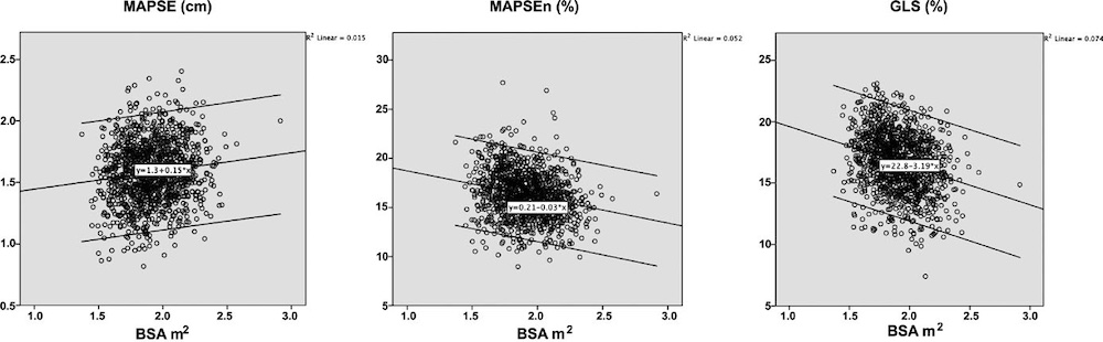
Relations of MAPSE, MAPSEn, and GLS to BSA. The figure shows a weak tendency of MAPSE to increase with increasing BSA, although the tendency is slight, and not enough to induce gender difference.
MAPSE was not significantly sex dependent (although with a trend of 0.1), while both GLS and normalised MAPSE were significantly higher in women (p=0.001), but by linear regression only BSA remained significant, so the sex differences are an effect of sex differences in size (18).

As shown by the boxplot, no significant gender differences in MAPSE, but in normalised MAPSE and GLS (women highest). All three measures are age dependent. Sex differences only due to differences in BSA, no independent contribution.
Sex dependency of GLS with higher values in women is also found in other studies with commercial speckle tracking (38, 39), indicating that this body size dependency is a general feature of GLS. Thus, it's the principle of normalising LV shortening for LV length in GLS, and not the method that induces the systematic error of increased and negative body size dependency.
Despite the fact that MAPSE correlates with SV, Global strain does not, and as this is by either method, so the effect seems to be systematic. Global strain on the other hand, correlates with EF (156).
In the HUNT3 study, using the geometrical model, Global MAPSE correlated with normalised global MAPSE (R = 0.86), GLS by segmental strain (R = 0.40), S' (R = 0.34), SV (R=0.25) and EF (R = 0.16), all p < 0.001). The two methods for GLS correlated with each other (R = 0.52), with S' (R = 0.26 and 0.44, respectively), with EF (R = 0.22 and 0.24), all p < 0.001). However, GLS by either method do not correlate with SV (156). The possible explanation is the previous finding that SV is related to both LV length and diameter, which are interrelated, while global LV strain only normalizes for LV length, thus introducing a systematic error as described above. The SV in this comparison, however, is derived from a geometrical model (65), which in itself may include a systematic error, but the concordant results between the two strain methods, as well as the maintained relation of SV with MAPSE and S’, supports this finding.
As SV and MAPSE increases with BSA, and GLS decreases with BSA, this lack of correlation was not surprising.
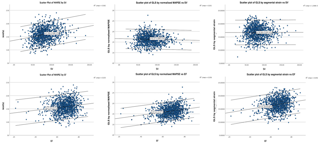
Diagrams, showing that MAPSE corelates with both EF and SV, while GLS by boith methods only correlates with EF, not BSA.
The reason for this is the relations to BSA, as explained above.
The long axis shortening and lengthening are thus related to annular displacement, and the strain curve is closely related to the relative volume (EF) curve. The strain rate is the first derivative of the displacement curve, just as the flow is the first derivative of volume. Thus, strasin and strain rate measures are myocyte length changes, which in turn are related to volume changes, not to contraction /contractility.
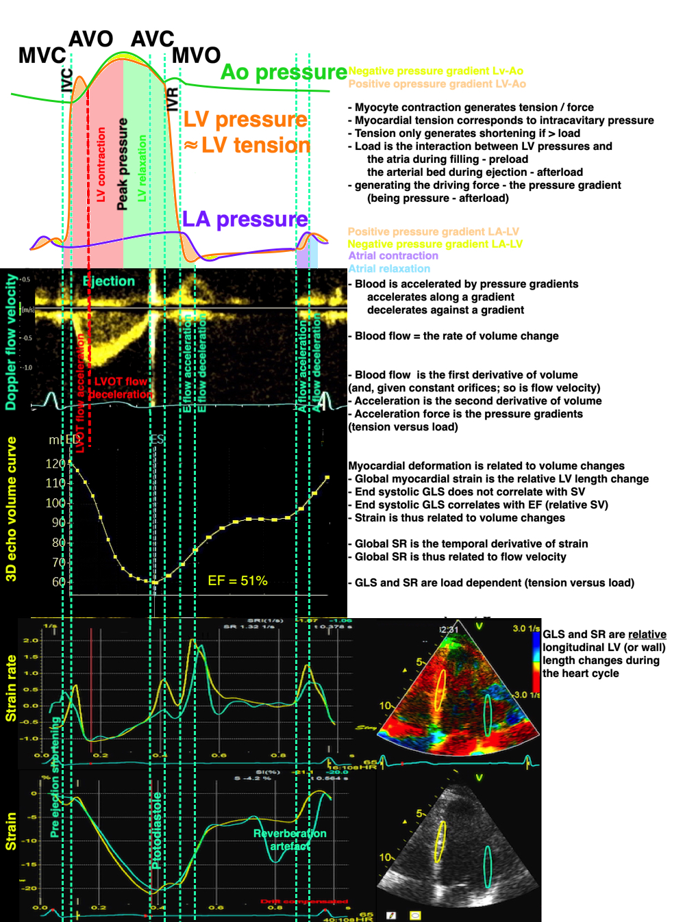
Relation of pressures, flow velocity, volumes, strain rate and strain. Strain and strain rate are measures related to relative volume changes (EF), and are thus functions of tension vs. load, andn not measures of contraction ( tension) nor contractility.
But what is the explanation of this apparently counterintuitive finding?
It is due to the fact that both LV length and diameter are related to BSA, and they are proportional (19). As the greater part of the SV is related to MAPSE × cross sectional annular outer area (radius squared), and as a larger ventricle has a larger cross sectional annular outer area, there can be a larger SV with the same MAPSE, so the adjustment of SV for a larger body and heart, do not necessitate an increase in MAPSE. But as the larger ventricle is longer, the strain denominator is bigger, and the absolute value of strain is lower, despite the unchanged MAPSE.
Diagram showing that as diameter (and cross sectional area) is larger in a longer ventricle, given the same MAPSE, SV can be higher with the same MAPSE, but GLS will be lower in absolute values.
Thus, BSA is a confounder for reduced GLS
We have seen that both MAPSE and GLS are reduced in reduced LV function. However, GLS is (numerically) reduced with incrfeased BSA. This means that BSA is a confounder for reduced GLS.
This is confirmed by a study showing that reduced MAPSE is a nbetter predictor for both events and death than GLS (282)..
As feature tracking tracks markers both longitudinally and transversally, the inward motion will give longitudinal shortening as well, even if there had been no true longitudinal shortening. This is thus an aertefact, as described here.
|
|
Speckle tracking image of the LV. The tracking bullets at the outer layer move least inwards in systole, the bullets at the endocardium move most, the mioddle row intermediate. Thus, there is a gradient of inward motion across the walls. | Hypothetical wall thickening, even without wall shortening. As the wall thickens, both the midwall (red unbroken) and the endocardial (blue unbroken) end diastolic lines move inwards. |
As shown here, transmural strain is relative wall thickening,
|
|
Transmural strain by M-mode. The M-mode measurement is more accurate than 2D measurements, but are only feasible in the septum and inferolateral (posterior) wall. | The average of septal and inferolateral wall should be used, as septal thickening is less than inferiolateral wall thickening, but then it's independent of symmetry assumptions |
It can be measured By M-mode (under some assumptions), By direct caliper measurements and by speckle tracking:
|
|
Top: direct caliper measurement of wall thickness (red lines). end diastolic and systolic thickness gives wall thickening. | Peak transmural strain values and strain curves from speckle tracking. |
Transmural strain is inversely related to wall thickening, as the myocardium is relatively incompressible as discussed here.
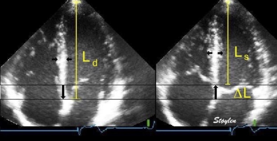
Deformation in systole. Left: end diastolic image, showing the end diastolic length (Ld = L0). During systole, the ventricle shortens with ![]() L, which gives (L = L0 -
L, which gives (L = L0 - ![]() L = Ls). But in order to conserve myocardial volume, the wall thickens at the same time, as shown by the horisontal arrows.
L = Ls). But in order to conserve myocardial volume, the wall thickens at the same time, as shown by the horisontal arrows.
Circumferential strain is equal to diameter shortening.
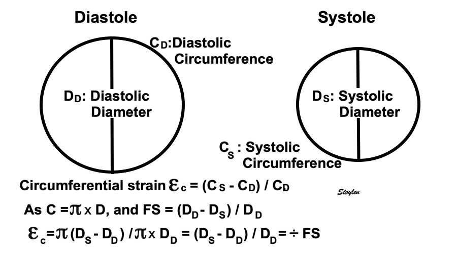
As diameter and circumference are proportional, fractional circumferential shortening and diameter shortening are equal.

As circumferential shortening equals diameter shortening, circumferential strains can be calculated from diameters, both in the outer, midwall and endocardial levels.As circumferences can be calculated from diameters, circumferential strains can be calculated from fractional shortening. Midwall and external circumferential strains were calculated from endocardial diameters and wall thicknesses.
In the HUNT study (7), Endocardial diameter was measured directly, and outer diameter (LVED) was calculated as LVED=LVID+IVS+LVPW both in diastole (LVEDd) and systole (LVEDs). Endocardial and external fractional shortening (FS) was calculated from internal and external diameters in diastole and systole in the ordinary way. Midwall FS was calculated from LVID + (2×1/2 WT) in systole and diastole, respectively.
Thus, there is a gradient of circumferential strain from the outer to the endocardial surface as discussed in detail here.
The circumferential strains in the HUNT study are given in the table below:
Circumferential strain can also be measured by speckle trackinbg:
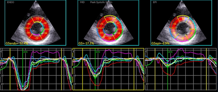
Circumferential peak systolic layer strains, in this example varying from - 32.4% in the endocardial layer via -17.3% in the midwall layer to - 6.9 in the outer layer.
It is very common to hear that as longitudinal function decrease with age or hypertrophy or whatever, the short axis function shows compensatory increase. Especially if EF is preserved. This mis conception artises from the confusion between cavity and wall measures. In the HUNT study, LV internal diameter, and fractional diameter shortening did not change significantly) with increasing age, while wall thickness increased, and wall thickening (transmural strain) decreased (19, 7) as shown in the table below.
The finding of the gradient of circumferential strain, has been interpreted as differential circumferential fibre function (shortening). However, this is faulty. In a thickening wall, both midwall and endocardial circumferences will move inward simply because of inward thickening, which is mainly due to longitudinal shortening, but also to circumferential shoertening, as this pushes the myocardium inwards, where there is less room in the circumferential direction, so it has to expand in the radial direction instead. And as there is a gradient of wall thickening, there will be a gradient of circumferential strain as well.
In the HUNT study, all strain components were found to be normally distributed.
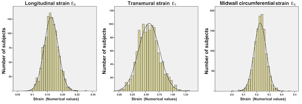
Normal distrubution of all three strains, with skewnesses of 0.17, 0.28 and −0.27 for εL, εT and εC, respectively
Larger speckle tracking studies gives mean and SD, so presumably the data are normally distributed, but makes no mention of the analysis of results for normality.
Total strain interdependence:
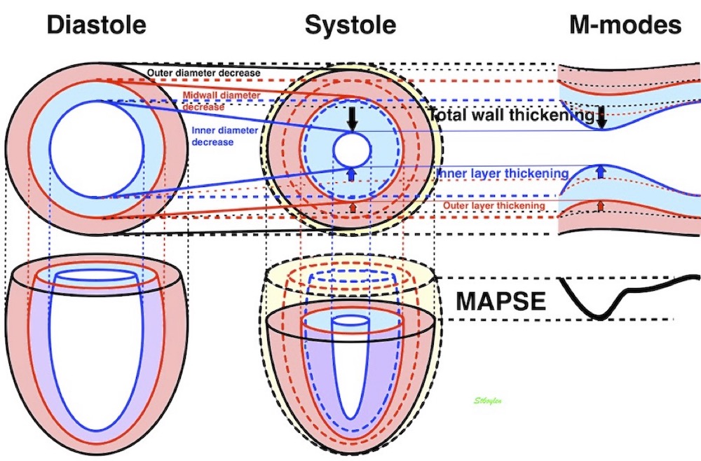
In the HUNT study, we found a clear decrease in all strain components with ageing (7):
Age (years) | εL (%) | Wall thickness (mm) | εT (= Wall thickening) (%) | LVIDD (mm) | Endo-card εC (=_FS) (%) | Midwall εC (%) | External εC (%) |
Women | |||||||
<40 | -18.1 (2.0) | 7.6 (1.3) | 45.8 (25,7) | 49.3 (4.2) | -36.6 (6.1) | -23.9 (4.1) | -14.1 (3.3) |
40 – 60 | -17.0 (2.2) | 8.2 (1.3) | 44.6 (23.7) | 48.8 (4.5) | -36.5 (6.9) | -23.2 (4.8) | -13.2 (4.2) |
> 60 | -14.8 (2.1) | 8.8 (1.4) | 43.7 (22.6) | 47.8 (4.8) | -36.0 (9.1) | -22.3 (5.6) | -12.1 (4,2) |
Total | -17.0 (2.4) | 8.2 (1.4) | 44.8 (24.1) | 48.8 (4.5) | -36.4 (7.1) | -23.2 (4.8) | -13.3 (4.0) |
Men | |||||||
<40 | -16.5 (2.0) | 9.0 (1.3) | 44.5 (19.9) | 53.5 (4.9) | -35.5 (6.9) | -22.4 (4.6) | -12.6 (3.7) |
40 – 60 | -15.4 (1.9) | 9.6 (1.4) | 44.1 (22.6) | 53.0 (5.5) | -35.8 (7.4) | -22.2 (4.9) | -12.2 (3.8) |
> 60 | - 14.9 (1.9) | 10.1 (1.5) | 41.3 (18.8) | 52.1 (6.4) | -36.0 (8.0) | -21.9 (5.2) | -11.8 (4.4) |
Total | - 15.5 (2.0) | 9.6 (1.5) | 43.5 (21.1) | 52.9 (5.6) | -35.8 (7.5) | -22.2 (4.9) | -12.2 (3.9) |
All | - 16.3 (2.4) | 8.8 (1.6) | 44.2 (22.7) | 50.8 (5.4) | -36.1 (7.3) | -22.7 (4.9) | -12.8 (4.0) |
Wall thickness, cavity diameter, Longitudinal, transmural and endocardial, midwall and outer circumferential strains by linear measurements from the HUNT3 study. Mean and standard deviations are given. LVIDD do not change with age. WT incrrases with age, Longitudinal transmural and external and midwall circumferential strains decline with increasing age, endocardial strain (AKA FS) do not.
The finding of unchanged LVIDD and FS has been confirmed before (32 - 37). And as we have found an unchenged EF with age, but no increase in any strain component, there is thus no compensatory increase in short axis function even with preserved EF (65), when short axis function is interpreted correctly.
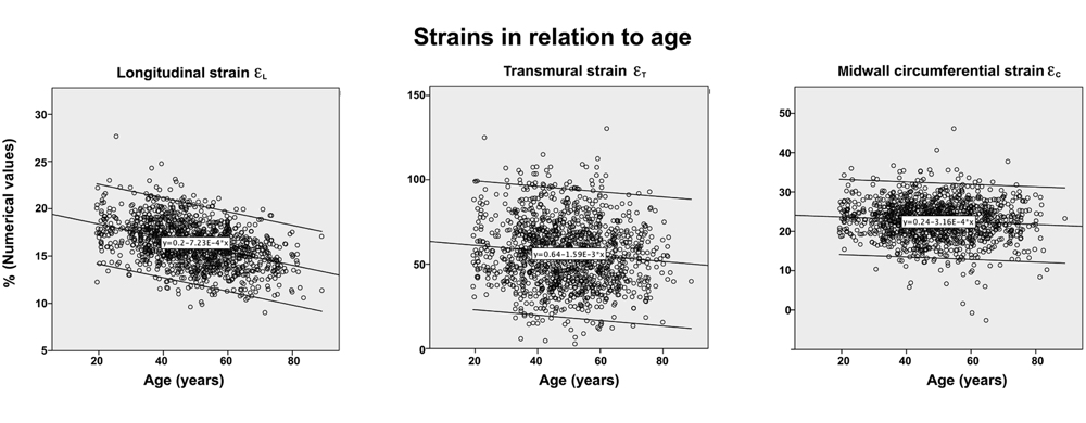
Again, the circumferential strains relate to diameter shortening. Thus endocardial strain, being equivalent to cavity fractional shortening will be preserved or even increase in concentric geometry, while
As we have seen in the HUNT study, the endocardial circumferential strain (which is the fractional diameter shortening), is unchanged with age, while the external circumferential strain (which is the real circumferential fibe shortening) decreases with age. As we have shown above, circumferential strain equals diameter shortening. This is true for both endocardial, midwall and outer circumferential strain:
However, the wall thickness increased with age, while LVIDd did not (19, 33, 34, 35). Despite the increasing wall thickness, the decrease with age was consistent, but considering that wall thickness will reduce transmural and circumferential strain relatively, this is logical.
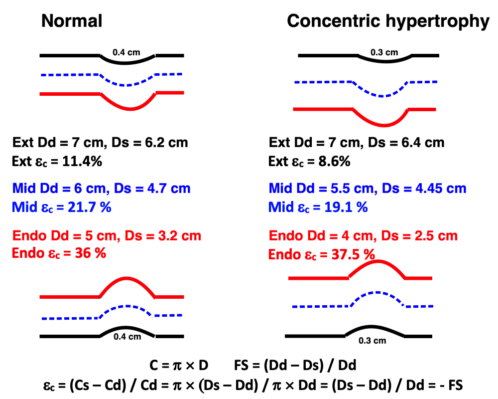
Same figure as above, schematic diagram of M-mode, illustrating the relation between cavity measures and wall measures of function. Here both endocardial (red), midwall (blue) and external (black) fractional shortening is shown. The circumferential shortening equals diameter shortening as shown below) For simplicty, the ventricle is assumed to be symmetric. Left, a normal ventricle with wall thickness of 1 cm, systolic wall thickening of 50% and a systolic 11% outer diameter reduction. This gives a fractional shortening of 36%. Right a concentric hypertrophic ventricle with reduced myocardial function. As the endocardial circumferential strain equals the FS, it is slightly increased. However, as wall thickening is reduced, both midwall and external circumferential strain is reduced.
This lack of compensatory transverse function is shown also in other studies of hypertrophy with HFpEF (80- 82) , all strain components are reduced simultaneously.
Thus, all measures are load dependent.
In addition:
Finally: In a working ventricle, much of the tension goes to develop increased pressure, not quantifialble by imaging per se.
The general definition of work is the force × the distance this force acts over. In this experimental setup: Work is total load (= force = tension) × shortening (W = F × s), as the isotonic contraction occurs at a constant load, where tension = load. In an isometric - istotonic twitch, this is only the dynamic work done in shortening. The static work done during isometric contraction is not counted in, as this builds up potential energy, which is then released during isotonic relaxation.
Thus, in work, load and shortening are inversely related, but work is still load dependent by the following argument: If force = 0, there will be no shortening, and work = 0. If load exceeds the maximal tension, there is also no shortening, and thus no external work being performed. If both are > 0, the work > 0 so the load dependency shows an inverted U - shape, that has been experimentally verified (79) as shown below.
The general definition of power is Work per time unit: P = W / t = F × s / t = F × v, i.e. force times velocity. As power is simply work per time, it is bound to follow the same inverted U shape as work, as experimentally verified (79) and shown below.
|
|
Effect of load on work and power. With increasing total load the muscle increases the work and power, by increasing the tension that is needed to overcome the increased load, despite decreased shortening, but only up to a peak. After that, increased load will decrease work and power by decreasing shortening, and at shortening = 0, W = 0. Increased preload increases shortening at all afterloads, and will increase both work and power. | Effect of inotropy on work and power. Inotropy will increase work at any given total load, by increasing shortening. It will also increase power, by increasing velocity of shortening. |
The general definition of work, is the pressure acting on the fluid, times the volume it is acting on, so force is equivalent to pressure, and shortening to volume. This is true both for the potential energy in a certain volume of fluid, and the work needed to move the volume at a certain pressure. Looking at the pressure volume curve, it is easily seen that the area of the curve is the myocardial work applied to the ejection of the stroke volume by the ventricle.
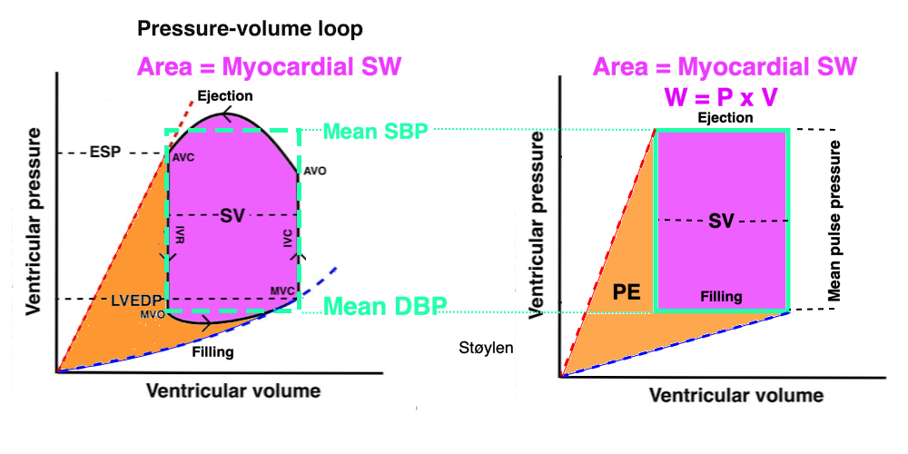
Myocardial work by the ventricle in ejecting a stroke volume. To make this more intuitive the pressure loop to the left is transformed to the right into a rectangular shape with the same area, where it is easy to see that the area is the height (equal to the mean pulse pressure × the width (the stroke volume). The magenta area is the external work, while the orange area is the potential energy developed by contraction and stored as elasticity, but released with relaxation.
This has also been confirmed experimentally (89) and clinically (90) by demonstrating a close relationship between PV-loop area and myocardial oxygen consumption. The height of the PV-loop is the SBP-LVDBP difference, which is the pressure myocardial work adds to the SV, the width is the SV. Mean SBP and mean LVDBP ((blue dotted rectangle), shows the relation in an easy way. GMsW is SV x (mean SBP - mean LVDBP).
The Global myocardial stroke work GMSW is thus closer to myocardial systolic performance, taking both stroke volume and pressure into consideration. It is thus SV × (Mean SBP - mean DBP).
A reasonable proxy could be SV × SBP, disregarding the shape of the systolic BP curve, eventual augmentation index and eventual elevated LVEDP.
However, GMSW will still be dependent on
|
|
|
Effect of preload. Increased preload (increased LVEDV - the right side of the curve moves right, the loop becomes wider), will, through the Frank-Starling balance increase stroke volume. This increased stroke volume will be ejected at the same pressure, thus returning to the same point on the ESPVR line. | Effect of afterload. Increased afterload (increased SBP moving the top of the curve upwards), will reduce the stroke volume. The end systolic point moves up the ESPVR line, shortening the width of the loop, i.e reduced SV. | Effect of inotropy. Inotropy shifts the ESPVR line to the left, thus increasing the force and LV emptying, increasing stroke volume through reduced LVESV, but also increasing the pressure, both through increased contractile force and increased volume being ejected into the vascular bed. |
Myocardial stroke work must necessarily behave like work in isolated muscle as described above. If the pressure = 0, no volume is ejected, and the work must be 0, if the pressure exceeds the maximal tension that can be developed, the volume also must be 0, and thus the work /afterload relation follows the same curve as the work in isolated muscle. However, the the theoretical situations of either load being higher than maximal power, resulting in zero SV, or SBP being zero, are both outside the physiological, and even pathophysiological range. Experiments, however, have shown LVSW to be both pre- and afterload dependent within the physiological (91) range, but LVSW increases with afterload.
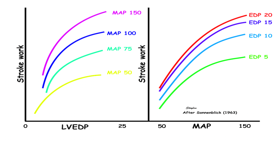
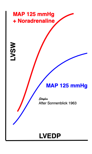
Curves from isolated heart experiments, showing that LVSW is both pre- and afterload dependent, within physiological pressure ranges, but while SV decreases with afterload, LVSW actually increases with afterload, and increases with inotropy when afterload is constant..
In acute changes:
GMW ![]() with
with ![]() contractility,
contractility, ![]() preload and
preload and ![]() SBP
SBP
GMW ![]() with
with ![]() contractility,
contractility, ![]() preload and
preload and ![]() SBP
SBP
SV ![]() with
with ![]() contractility,
contractility, ![]() preload and
preload and ![]() SBP
SBP
SV ![]() with
with ![]() contractility,
contractility, ![]() preload and
preload and ![]() SBP
SBP
Stroke volume increases by contractile tension. this means that at unchanged afterload GSW increases with preload, it increases with inotropy, and decreases with reduced contractility. But SV also decreases with increasing afterload, although GSW increases, so GSW is thus positively afterload dependent, while the other measures of contractile tension are not.
In the clinical situation, this means that SW will increase in afterloaded situations and disease, but decrease with myocardial failure.
This means that SW, increasing with increasing afterload (and preload) is a measure of LV performance, but not closer to the contractility measures (SV, EF, strain), which decrease with increasing load. Nor is it a contractility measure, which is load independent. It does, however increase with inotropy (91). Myocardial work is thus myocardial energy expenditure, which is relative to the performance and demand put on the muscle by load. Thus Global myocardial work is exactly that, the work performed by the ventricle in relation to both demand and capacity.
Myocardial work is thus equal to myocardial energy expenditure, which is relative to the demand put on the muscle by load , and the performance in response to this demand, both by preload and by inotropy. Thus it is a mixture of force supply and demand, and even though GMSW is a closer measure of the total myocardial performance, it is not closer to a measure of contractility, in fact, it is not about contractility at all, but about myocardial energy expenditure.
In chronic changes; As neither EDV nor EF enter into the equation, GMSW is EF independent, and not a contractility measure at all.
Ventricles with EDV of 300 ml, 150 ml or 100 ml, with EF of 25%, 50% and 75%, respectively, will all have SV of 100 ml, and expend the same energy (same GMSW) at the same SBP, but the contractilities are vastly different.
Thus SW depends only on SV and BP, regardless of EF, so it isn't about contractility at all, in dilated ventricles.
In the clinical situation, this means that SW will increase in afterloaded situations like aortic stenosis and hypertension, and thus increased GMSW is deleterious, but it will decrease with myocardial failure, which is also deleterious. Decreased SW is thus negative if it is due to reduced SV, but not if it is due to reduced BP within normal range.
Increased SW is negative if caused by increased BP above normal range.
Myocardial power = Work / time. This means that it can be calculated as LVSW / ejection time, which is mean SBP × SV / ejection time, or approximated by SBP × SV / ejection time. As with myocardial work this has to be load dependent as illustrated above. However, as shortening velocity also is inotropy dependent, with higher contractility, the time will be less, and the power higher for any given work.
Another approximation will be MAP × SV / RR-interval, as the SV is the same in aorta as in the LVOT, but smeared out over the full heart cycle, where the work done in systole to dilate the aorta is recovered in diastole for the diastolic aorta flow. And this again, can be translated to MAP × CO, which is the same value, although this has been named cardiac power output.
Looking at two different ventricles with different contractility performing the same work, it seems reasonable that the ventricle with best contractility may perform the work with higher velocity, i.e. in shorter time, and thus power may show difference in contractility where work may not.
Difference between power and work. At the end of the road, the two trucks, carrying the same load, the same distance, will have performed the same work (W = F x d). However, the lower truck, with a bigger (stronger) engine, is able to run at a higher speed with the same load, and thus perorm the work in a shorter time, i.e. with a higher power.
As the pressure in myocardial work is the intraventricular systolic - diastolic pressure, it is at the outset dependent on invasive LV pressures. However, systolic pressure can be estimated from systolic brachial pressure, as a proxy for mean systolic pressure.
However, It does not take pressure augmentation by reflected waves into account, which may underestimate the pressure, but on the other hand, using peak pressure instead of mean pressure will overestimate the systolic pressure, and thus the two systematic errors go in opposite directions.
Diastolic pressure mus be estimated, however.
A proxy for mean SBP - mean LVDBP has been MAP, giving GMSW = SV x MAP.
Various method for estimating DBP have been tried as well, based on models, or on databases. However, model estimates are only valid for the population where they are validated, and especially estimating of diastolic pressure is not valid in ischemia without having been validated in ischemic models or populations.
E/e' has been applied as a correction for elevated DBP. ref. However, while this is a marker for elevated LAP, and thus LV mid diastolic pressure, it is not a linear relation.
A new measure of global myocardial work, based on estimated Global strain - pressure Loops, has aroused interest lately. I suspect that it is the same as for regional vs global strain, while regional strain is noise sensitive, research turned to global strain, which is more robust, but which, however, probably do not add anything to MAPSE (18).
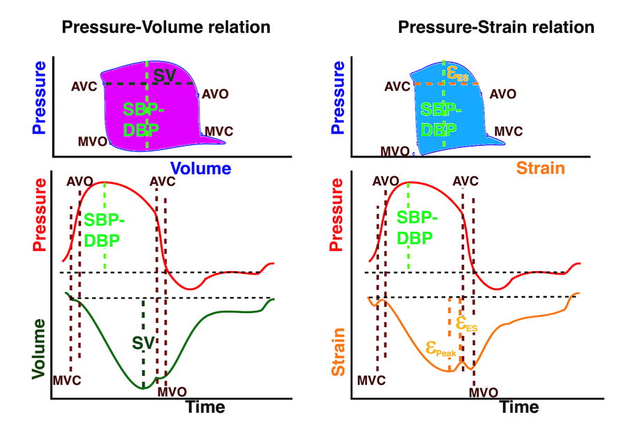
Left: Conventional pressure volume relation, the volume curve taken from a MUGA scan. The area in the PV loop is the myocardial work, and the loop is defined by the DBP-SBP-difference giving the height of the loop, while the SV is the width of the loop at the time of AVC. However, the pressures are based on estimates, if not measured invasively. Right pressure-strain relation. Since the strain and volume curves are similar, so would pressure-strain and PV-loops be. The height of the loop would be the same, derived from the DBP-SBP-difference, but the width of the loop is defined by the end systolic strain at the AVC. As myocardial work would be expected to be lower, the loop has to be narrower if they are drawn to scale, representing only about 75% of global myocardial work, and would depend on the strain correlating with the SV.
The pressure-strain curve is equivalent to the work derived from the tension length relation. But as the whole ventricle is a volume, the two measures are not the same. Firstly longitudinal strain only accounts for between 60 and 80% of stroke volume, and the area of the pressure strain loop would be correspondingly lower, except that speckle tracking strain will over estimate longitudinal strain. Secondly, as work relates to volume, the work is the energy needed to eject a cartain volume, W = P × V. Work = Force × distance, Pressure = Force / Area, so W = P × A × d = P × V.
GLS only considers the longitudinal shortening, and thus disregards the surface area (Laplace's law). Thus, GLS cannot replace SV. We have also shown that GLS actually do not correlate with SV, only with EF(156),also due to the systematic error that GLS only corrects for length, not for both length and diameter. This means that the validity of GMW based on GLS is in question.
GMW on the other hand is EF independent, while GLS correlates with EF. Thus, MAPSE correlates both with SV and EF, while GLS only correlate with EF, not SV, and GLS is not a proxy for SV in GMW. In addition, substituting P x V (area x length) with P x Length, is not in line with physics. so basically there are serious concerns about the validity of strain based GMW.
It would rather be an equivalent to EF × BP.
It's important, however, to realise that prognostic outcome studies do not define things or validate proposed pathophysiology of a parameter, they are at best supportive. There will always be confounders/ competing risks, and even if an index is valid only for a subset of cardiac patients, it may still have an overall statistical impact.
The AV-plane moves towards the apex in systole, causing longitudinal compression of both ventricles, but als a concomitant expansion of the atria during the ejection phase.
The relative constancy (but not total as explained here) of the outer heart contour means there is a reciprocal relation between the ventricular and atrial volumes.
There is a reciprocal relation between the atrial and ventricular volumes, as both are related to the AV-plane motion.
- which means that the apical motion of the AV-plane compresses the ventricle longitudinally, but also expands the atrium:
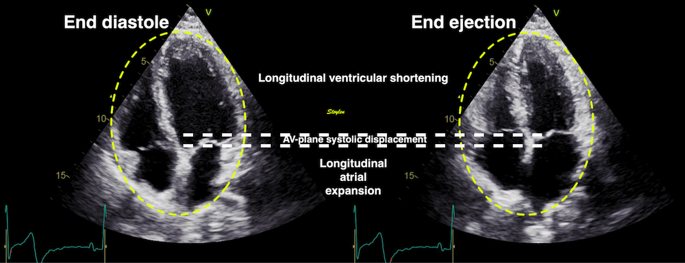
The M-mode of the AV plane shows the atrial expansion:
M-modes through the mitral ring (septasl - left and lateral - right), showing that there is shortening of the ventricles and concomitant expansion of the atria throughout systole
Thus, we see than there is atrial expansion during the whole systole, but peak systolic flow is concomitant with peak AV-plane velocity, during early ejection, and the venous flow decreases as the AV-plane velocity decreases.

Comparing PV flow with LVOT flow and tissue Doppler. Reducing clutter filter, the tissue signals can be see as described here. Here compared with the septal TVI curves (aligned by ECG - cyan lines). In LVOT, there is a near perfect match in timing of the TVI signal from clutter, and the TVI signal from the adjacent mitral ring. It also coincides fairly closely to peak flow velocity, indicating peak active contraction. Thus the tissue Doppler clearly shows the declining rate of annular motion and atrial expansion.
Ventricular longitudinal systolic shortening thus causes pressure increases during early and late filling (53) as well as atrial expansion, drawing systolic inflow to both atria, the S-wave (16, 59 - 61), simultaneous ventricular emptying and atrial filling of the heart driven by ventricular contraction (9). Thus, most of the filling volume to the ventricles, is a function of the AV-plane pumping.

The AV-plane moves towards the apex in systole, causing longitudinal compression of both ventricles, but als a concomityant expansion of the atria during the ejection phase .
This means, that during ventricular longitudinal systolic shortening in the ejection phase, the atria expands, and aspirate blood from the large systemic vains to the right atrium, and from the pulmonary veins to the left atrium, the S-wave as can be demonstrated by Doppler (59, 60).

Pulmonary venous flow visualised with CFM. The systolic and diastolic phases of inflow to the atrium are evident.
Still frames from the same loop, showing ejection (left), early filling (middle) and atrial systole (right). Here, a weak signal of atrial reverse flow is also visible.

Left: Colour M-mode showing the apical motion of the AV plane during ejection by the white dotted line, the concomitant ejection from the ventricle (blue colour over the AV plane) and the systolic inflow into the left atrium, the S-wave (red colour under the AV-plane). Right pw Doppler, top showing the systolic ejection from the ventricle, bottom showing the pulmonary venous inflow to the left atrium. The S-wave is the systolic component.
Thus, there is simultaneous ventricular emptying and atrial filling of the heart driven by ventricular longitudinal contraction (9). Direct measurement by MR have shown that the AV-plane contribution is closer to 60% for the LV, but ca 80% for the RV (66, 67,68), although a study of LV filling found that systole contributed 70% to cardiac filling (9), which should be equal to the ejected volume unless there is concomitant systolic atrial expansion also. The total cardiac volume, however, has been shown to decrease during ejection, meaning that the ventricles are compressed more than the atria expand, due to the transverse compression of the ventricles (62, 63).
The pattern of venous inflow to the right and left atria are similar (157).
|
|
Atrial /red), left ventricular (blue), Pulmonary venous (magenta) and pulmonary artery (green) pressure curves. a: atrial pressure rise during atrial contraction. z: pressure decline after a. c: Initial atrial pressure rise at start systole x: pressure decline during LV ejection V: pressure rise at end ejection. | AV-plane motion, tracing the atrial expansion during LV ejection, and atrial compression during ealry and late filling. |
This means that the systolic atrial filling is to a large degree dependent on ventricular function. Looking at the atrial pressure curves, atrial contraction results in a pressure rise, the a-wave, the c wave at the start of systole may be related to pre ejection contraction of the ventricles with open AV valves, and possibly to bulging of the AV valve cusps into the atria during IVC. Aftyer the c-weave there is pressure declie (x-descent), due to the expansion of the atria by the AV-plane motion during the ejection. At the end of ejection, the velocity of AV-plane descent declines, so the inflow exceeds the atrial expansion, generating pressure increase, the v-wave. This may also be driven by the propagation of pulmonary pressure.
Pressure gradients from PV to LA from the figure above, compared to a standard flow velocity curve. The pressure gradient is negative (magenta) during the a wave, driving flow backwards (A), and positive during the rest of the cycle (violet), driving flow forward. Looking only at the arial curvem, however, this very closely mirrors the pulmonary flow velocity profile. | Looking at the atrial pressure alone, it can be seen that pulmonary venous flow is almost perfectly mirroring the atrial pressure curve alone. Pressure peaks correspond to velocity nadirs, pressure troughs to velocity peaks, pressure decrease to acceleration and pressure increase to deceleration. |
The z descent may be due to atrial relaxation, while the c wave may be ventricular pre ejection contraction causing atrial pressure increase, and the ventricular iVC contraction causing some bulging of the leaflets into the atria.
|
|
Pulmonary venous flow. The systolic flow can here be seen as two component, where s1 corresonds to the pressure drop between a and c waves (the z descent), which may be due to atrial relaxation (i.e. the S wave is split by the c-wave), so the C-wave maand the notch may be the ventricular contraction during pre ejection and IVC ), and the S2 being the x-descent after the c-wave. | Another common normal pattern of pulmonary venous flow, where the split of the S-wave in not apparent. |
Thus: During x-descent, we have atrial volume increase (positive dV) and pressure decrease (negative dP). This means that there is negative compliance C = dV / dP. Negative compliance is equivalent with suction, so the whole of the x-descent represents suction, generated by the AV-plane descent.
The main contributor to the volume change is the AV_plane motion, while the outer contour of the heart is less variant (11 - 16, 64 - 67). Simultaneous ventricular emptying and atrial filling in systole are driven by ventricular longitudinal contraction (9), i.e. AV-plane motion. This is evident from the previous paragraph.
This, of course must mean that the atrium also deforms through the heart cycle.
However, there is a common misconception that while ventricular strain relates to ventricular function, atrial strain relates to atrial function. However, both relates to AV-plane motion:

Systolic AV-plane motion. During ejection, there is longitudinal compression of the ventricles, and expansion of the atria, during early and late filling there are longitudinal expansion of the ventricles and compression of the atria.
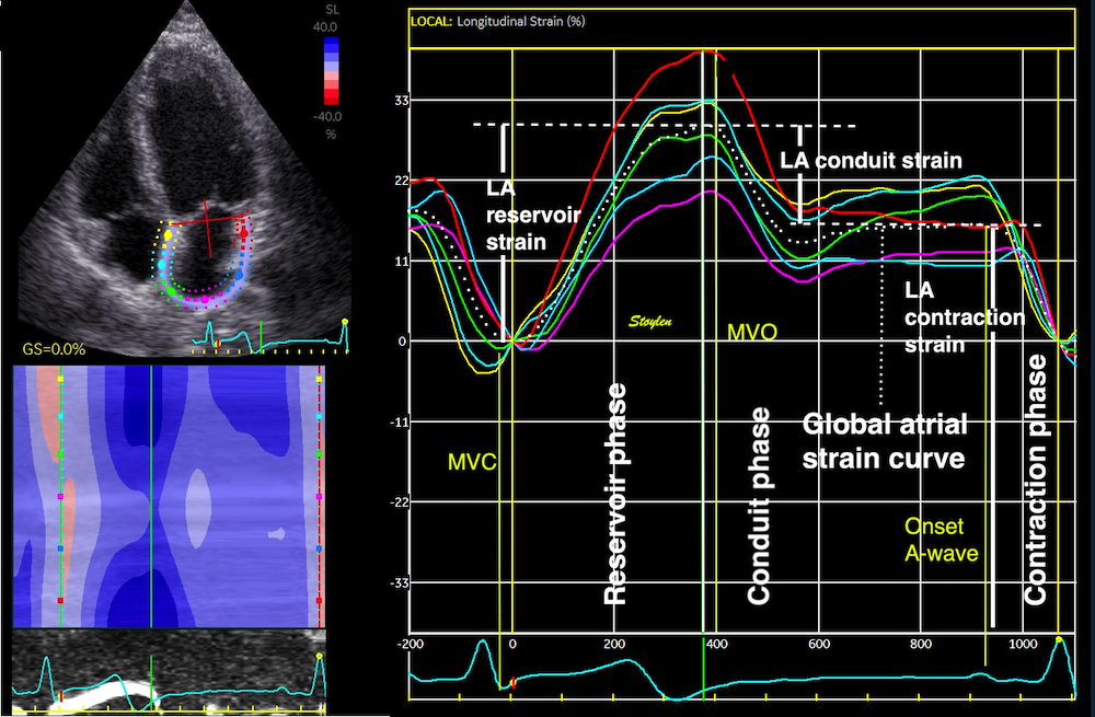
Longitudinal atrial strain by speckle tracking. The curves are obtained by drawing an ROI through the LA wall, instead of the ventricles. Thus, the atrial strain is the relative change in LA wall length through the heart cycle. As the atrium is expanded in systole, (elongation) this means the strain is positive. Remark the strong similarity of the curve to the mitral plane motion curve. There are three phases as recommended by present guidelines: LA "reservoir strain", LA "conduit strain" and LA contractile strain as shown in the figure.
However, both ventricular systolic contraction and atrial expansion are simultaneous and mediated by the AV plane motion, as shown above.This, of course is because both are reflections of the mitral annulus motion, the long axis function of the heart. The mitral annular motion from the same patient, shown by TDI, has the same shape.
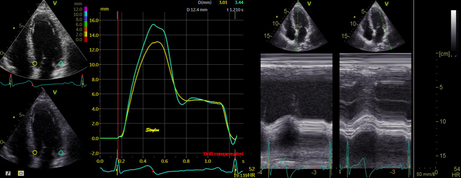
Mitral annular displacement, shown both by tissue Doppler and M-mode, seing they are nearly identical in shape to the atrial strain curves.

Reciprocal LA strain and LV strain curves derived from the same heartbeat.
And this reciprocal interdependence is also demonstrated. The most important determonant of LA strain, is thus LV strain as found when they are compared directly (69, 70).LA and LV strain curves correlte with R2 > 0.90 for the whole cardiac cycle, and R2 > 0.97 for its phases (70).
The atrial deformation during the heart cycle is (71)
However, this means that the the same AV-plane motion is considered as ventricular function when looked at from the ventricular side, and atrial function when looked at from the atrial side, which is obviously nonsense.
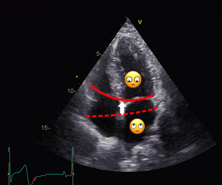
It's slightly strange to see the same events (periods) change physiological interpretation looking from the atrium towards the AV-plane, instead of from the ventricle.
This means that both systolic ventricular strain (during ejection) and LA "reservoir strain" are AV-plane motion with MAPSE as numerator, and they are also simultaneous. It seems fairly meaningless to consider the same event as ventricular function looking at the AV-plane from the ventricle, and as atrial function from the atrium.
Thus atrial strain as ventricular strain, is intimately related to the AV-plane motion:

Atrial strain vs AV-plane motion in the same subject. As we see, the atrial strain phases of reservoir, conduit and contraction, are the same AV-plane motion as the ventricular ejection, early and late filling.
Ventricular systolic strain, is shortening per length unit, i.e. relative shortening of the LV (wall). Even though there is no definite gold standard, and values vary by method, this is in line with the original Lagrangian definition of strain,
![]()
and the physiological interpretation is a measure of myocardial systolic function.
The LV systolic strain is the MAPSE normalised for the LV wall length, while the LA reservoir strain during the ejection is MAPSE normalised for LA wall length (LAWL). Thus, they share the same numerator, and cannot be independent, but in fact is highly interdependent with an R2 of 0.95 (70).
The mitral annular-plane motion (MAPSE) is the main determinant of the global LV systolic function (65, 66, 67). This means that reduced MAPSE will result in reduced LA strain as well as LV strain. The correct name for the atrial strain should thus be "atrial strain during ejection. Atrial strain during ventricular ejection, is the relative elongation of the atrial or atrial wall by ventricular shortening, but what's the physiological interpretation of that?
It has been termed the "reservoir atrial function or Left atrial reservoir strain (LARS). The connotation of this is that it should be some measure related to atrial volume expansion, or compliance.
However, the event is powered by the longitudinal ventricular myocardial contraction, which expands the atria, and aspirate blood from the veins (9). Thus, MAPSE is the numerator of LA reservoir strain, i.e. a measure of LV function.
The term "LA reservoir function" is a misnomer, and LA strain should rather be termed "LA strain during ventricular systole". The atrial strain during ejection, is thus a composite of LV systolic function as numerator, and atrial size as denominator, so again this composite measure contains inherent confounders, and being so interwoven with LV function, and with sconfounders, the real clinical value of this is dubious.
This means that reduced LV function must give reduced LA strain, and ventricular function is a confounder, or maybe even the most important determinant for LA strain during ejection. And MAPSE is reduced both in HFrEF and HFpEF.
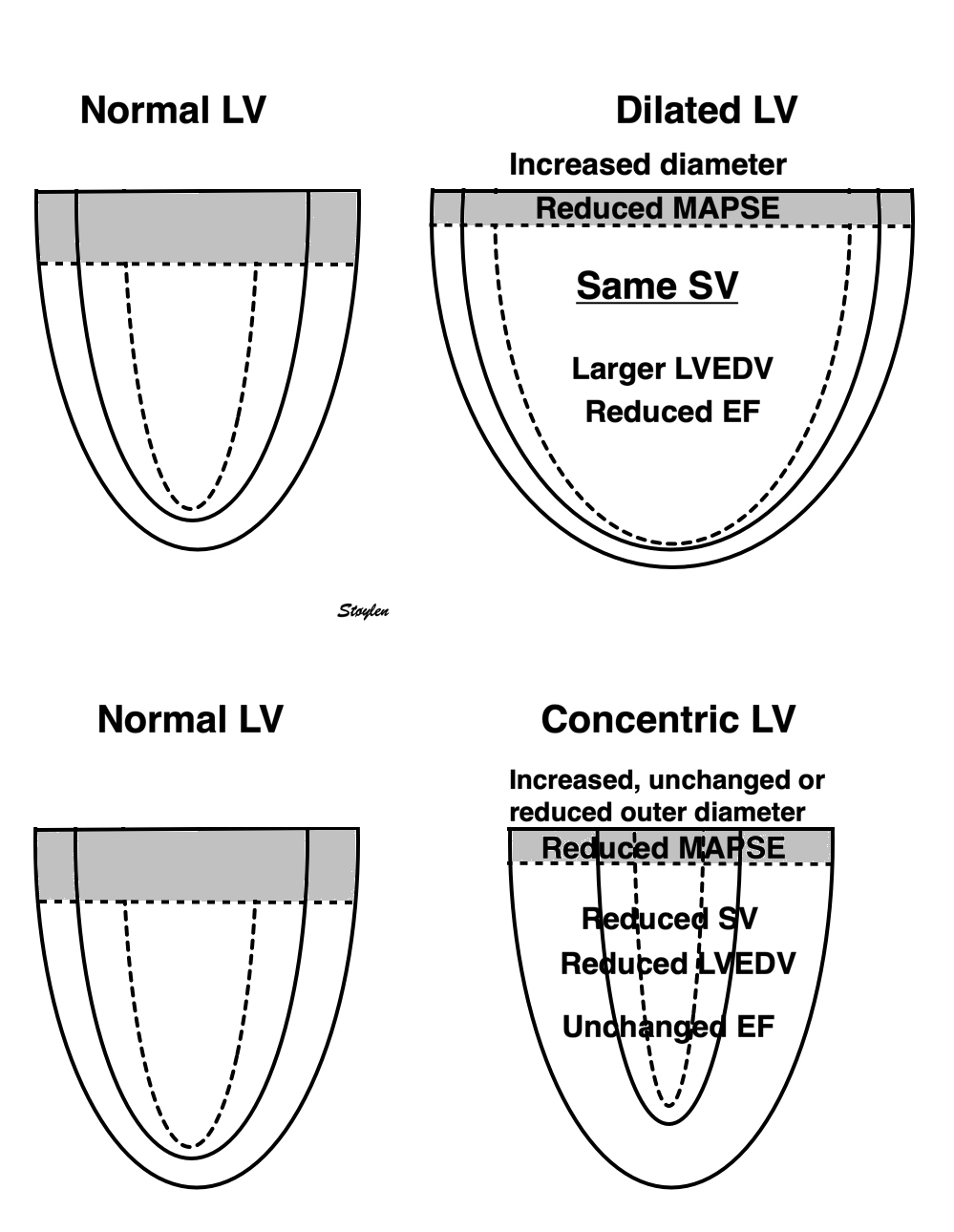
Diagram of MAPSE in relation to a dilated LV with reduced EF (HFrEF (top). When the left ventricle dilates, both the volume and diameter increases, and the stroke volume can be maintained by a smaller fraction (Ejection fraction) of the total (end diastolic) volume. As the stroke volume is proportional with the MAPSE x outer area, as discussed above, the SV also can be maintained with a lower MAPSE and a larger diameter, and there will be a near linear relation between reduction in EF and MAPSE. In concentric hypertrophy the LVEDV is reduced, and unable to generate the same SV. But as both LVEDV and SV is reduced, the EF may be preserved (HFrEF). The outer diameter may be increased, unchanged or reduced, depending on the pattern of wall thickness increase. Still the SV is proportional to the MAPSE x area, as discussed above, there will be a linear relation between the decrease in MAPSE and SV.
LARS is thus affected by all factors affecting MAPSE; Inotropy, preload, afterload, LV myocardial failure, fibrosis, deposition disease, which all are confounders in relation to atrial function.
Interpreting LA reservoir strain (LARS) as a measure of LA stiffness, is thus a misunderstanding, shifting the perspective of MAPSE doesn't change the interpretion from ventricular to atrial function.
Recently, a measure called LA stiffness index (LASI) has been introduced as LASI = (E/e’)/LARS.
If LARS had been a measure of LA stiffness, which it isn’t, the ratio of E/e’ divided by LARS would have been a measure of LA elastance, so it isn’t. Instead it simply adds more confounders.
LASI = (E/e') / LARS = (E/e') / (MAPSE/LAWL) = (E × LAWL) / (MAPSE × e'), meaning that:
LASI increases both with good diastolic function, restrictive filling, reduced LV function and increased atrial size, but decreases with delayed relaxation and reduced e'.
Increased LA size, being the denomintor for LA strain, so any condition that enlarges LA, will reduce LARS.. But this is an association, not a causal relationship.
Primary LA remodelling, of course may lead to increased LA size, and thus reduced LA strain, even with preserved LV function and MAPSE. Thus, AF then is the cause, and not the effect of decreased LA strain, and the association of reduced LARS and AF is not causal, but revere causality.
.
Increased LA pressure will also give atrial dilation, and thus decreased LARS. As reduced LV function (both HFrEF and HFpEF have reduced MAPSE) is the commonest cause of elevated LA pressure, and LA size is a consequence of elevated LA pressure, LA strain during systole is a measure of LV function, not LA function, and systolic ventricular function is a confounder for tha LA reservoir strain.
Looking at the ejection, the delay before peak ejection velocity (acceleration time) is evident. At the same time, the AV-plane can be seen to move towards apex, and the systolic venous inflow to the left atrium is also evident.
It is evident that is general, the intraventricular flow and AV-plane motions occur in opposite directions.
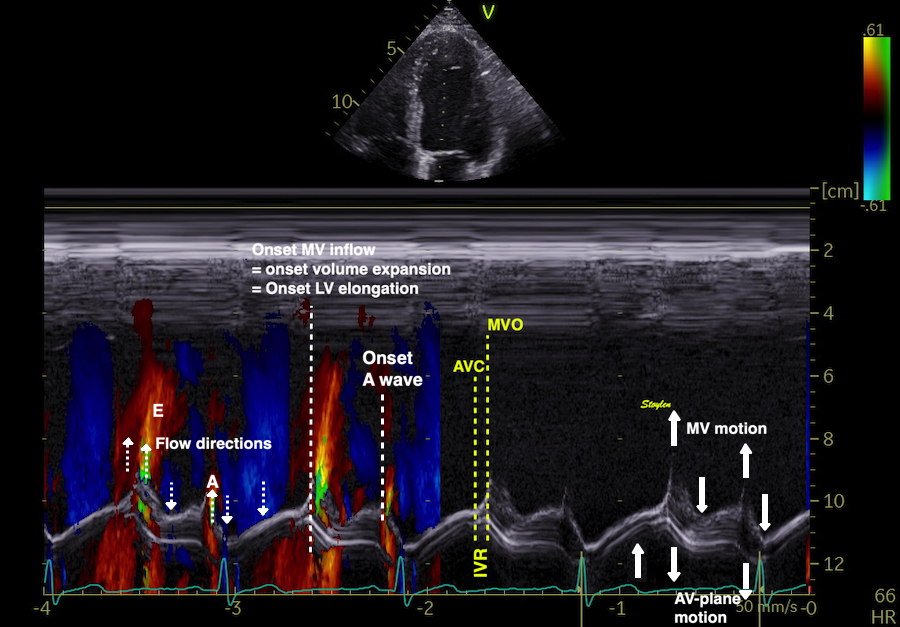
Colour M-mode showing theat during ejection, the flow is directed towards the base (emptying - out of the LV), while the AV-plane motion is directed toward the apex (longitudinal shortening of the LV. Both are manifestations of the reduction of the LV volume.
This, however vil initiate vortex formation in the LV even during ejection, by pushing blood towards the apex outside the column of blood moving out of the LVOT.:
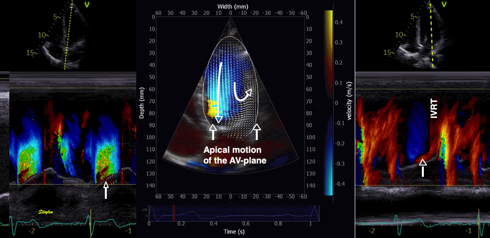
The colour M-mode to the left shows simultaneous ejection of the apical motion of the ventricular base, while the 2D image shows that some of the recruited flow is directed laterally and apical. Basally flowing blood meeting the mitral leaflets, will either be forced to converge towards the LVOT, or towards the lateral wall. The latter, however, will meet the apically moving leaflets, so some blood will receive an apical momentum from the moving AV-plane. Image courtesy of Annichen S Daae. The right M-mode shows how the apically moving mitral leaflet (ventricular base) pushes some blood in the apical direction, creating a new apical momentum, even before IVR.
This apical gradient thus increases, creating a transient peak vorticity, but as the ejection flow at the same time decreases, the vorticity decreases again. The apical momentum, however, remains, adding to the apical flow momentum created during IVR,
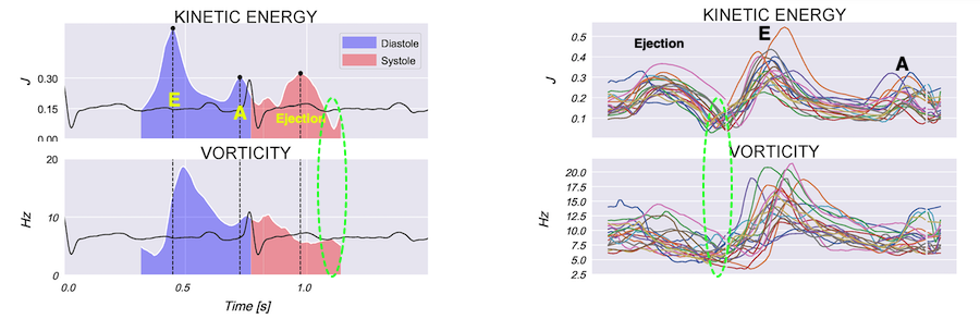
Vorticity and kinetic energy, plot, showing little vorticity during ejection. During late ejection, KE decreases while vorticity increases, indicationg new vortec formation. Images courtesy of Morten S Wigen.
Thus, the systolic AV-plane motion during ejection also takes part in the generation of the apical momentum that is further generated during IVR.
The concept that the heart functions as a double pump, with the atrioventricular plane as a piston, rather than pumping by squeezing, is indeed a concept dating back to Leonardo da Vinci. In 1932, Hamilton and Rompf argued from experimental studies that the heart worked mainly by the movement of the atrioventricular plane toward apex in systole, away from apex in diastole, while the apex remained stationary and the outer contour of the heart relatively constant .
Their hypothesis was confirmed by Hoffman and Ritmann in CT studies in dogs in 1985, showing a stationary apex, constant outer contour and motion of the AV-plane. They also stressed that this mode of action minimised the energy expenditure as the ventricular volume rediction in systole moves blood into the heart, rather than moving the surrounding tissue during systole. If the heart should be pumping by inward squeezing, reducing the outer contour of the heart this would be unfavourable energetics, as this means moving the surrounding tissue (lungs and mediastinum) inward by each heartbeat, without regaining this energy in diastole. Stig Lundbäck, in a series of elegant human studies using both gated myocardial scintigraphy, echocardiography and coronary angiography (Demonstrating the outer heart contour by tangential cine angiograms of the LAD), documented the invariant outer contour and the AV-plane mode of working (12 - 14) .

There is a reciprocal relation between the atrial and ventricular volumes, so both systole and diastole are related to the AV-plane motion.
This is energetically feasible, as the work used to decrease the volume, in additon to ejection, also moves the blood from the veins into the atria. If the heart had worked by squeezing changing outer contour to a high degree, the work would have been used to shift the rest of the thoracic contents especially lungs inwards in each systole, work that would have been wasted.
Ventricular longitudinal systolic shortening thus causes pressure increases during early and late filling (53) as well as atrial expansion, drawing systolic inflow to both atria, the S-wave (16, 59 - 61), simultaneous ventricular emptying and atrial filling of the heart driven by ventricular contraction (9). Thus, most of the filling volume to the ventricles, is a function of the AV-plane pumping.
However, this model needs modification.
Firstly, studies have shown a contribution of outer contour decrease to the stroke volume (62, 63, 65).
Secondly, the simplified eggshell model is not consistent with the presence of either atrioventricular flow, nor venous inflow.
|
|
If the moving AV-plane is responsible for the ejection, as well as the full expansion of the atria, the ejection volume from the ventricles and the venous inflow volume would be equal, there would be no volume changes of the heart. | In diastole, the recoil of the AV-plane would simply shrink the atria and expand the ventricles to ventricularise the volume that had been atrialised during systole, and the volume remain stationary during the shift, with no atrioventricular flow and this would be the effect of the total diastole. Also this would mean that there would be no venous inflow to the atria, as there is no total volume change. |
However, taking into account the fact that the mitral annulus is smaller than the mitral ring, the annulus will not be able to grab the whole of the atrialised volume, meaning that the remainder gives rise to atrioventricular flow. Thus, the difference between the annulus diameter and and the ring diameter is consistent with the presence of transmitral E and A flow. However, in a heart with total invariant outer contour, the atrial filling in systole would be equal to the ventricular emptying, and so there would be no further atrial filling in diastole. However, the presence of inflow to both atria during diastole (the D-wave) (16, 59 - 61), shows that the systolic atrial filling has to be less than the ventricular emptying, and so there is additional atrial filling (venous inflow) during early diastole, as shown below. The systolic fraction of the total LV stroke volume has been quantified to about 70% of the total SV in healthy subjects (9). (This however, does seem to place the longitudinal contribution to the LVSV closer to 70% than 60%, unless there is systolic transverse expansion of the atria as well as longitudinal.)
This is consistent with the findings of a ventricular outer volume decrease by MR, (62, 63), and by echo (7, 64, 65) due to transverse shortening
The diastolic function is the interplay between
As myocardial contraction do not equal shortening, do myocardial relaxation not equal lengthening, except in completely unloaded experiments in isolated cells or muscle.
The rate of relaxation is governed by the dissolution of actin - myosin cross bridges, which again relates to the rate of removal of calcium from the cytoplasm. This dissolution of the cross bridges releases tension. But this is an active, energy consuming process, due to the active calcium transport into the sarcoplasmatic reticulum. The contractile apparatus itself has no mechanism for sarcomere lengthening, only shortening.
The lengthening itself has no active mechanical component in the contractile apparatus itself, and must be due to elasticity, i.e. stored elastic energy from systole.
In the free cell and in isolated muscle, elongation starts at start of tension release (- decrease), and as the cell also elongates, there must be elastic energy stored in the cell itself.
In the intact heart, , however, tension decrease starts at the start of pressure decrease, this means before mid ejection.
|
|
|
Image of beating isolated myocyte, prepared so the cell fluoresces with the presence of free calcium in the cytoplasm. In systole the cell can be seen to increase free calcium and simultanously shorten. In the cellular diastole, the cell can be seen to elongate, and simultaneously free calcium disappears from the cytoplasm. Image courtesy of Ph.D. Tomas Stølen, cardiac exercise research group (CERG), Dept. of Circulation and Medical Imaging, Norwegian University of Science and technology. | Excitation-tension diagram. The Action potential triggers the influx of calcium, which triggers further release of Ca2+from sarcoplasmatic reticulum. Calcium binds to troponin, and allows activated (by ATP) myosin heads to bind to troponin sites on actin (cross bridge forming) and release energy, causing the filaments to slide along each other, as long as there is a high calcium concentration in the cytoplasm. As the cell membrane repolarised, this triggers the removal of calcium from the cytoplasm, mainly by the SERCA pumping it into the sarcoplasmatic reticulum again. The removal of free calcium is an energy (ATP) demanding, active transport of calcium into the sarcoplasmatic reticulum by SERCA.Thus, obviusly, both contraction and relaxation are ATP demanding processes, and energy depletion will affect both. | Sarcomere diagram. Sarcomere shortening occurs in systole by the calcium faciltating binding of the myosin heads to the actin filaments whilt released energy causes the heads to rotate, pulling the actin filaments along the myosin. and hence, shortens the sarcomere. Removal of calcium, however, only releases the bindings which releases tension. But this means that there is no inherent mechanism that pushes the actin the other way, (even if there had been reverse rotation (which occurs in the poresence of ATP), as the bindings are disolved. |
In the intact heart, flow acceleration occurs during positive LV-Ao gradient, and the end of this positive gradient occurs at peak flow, which is also the peak rate of volume decrease, of course. Pressure crossover to a negative LV-Ao gradient marks the start of flow deceleration, as explained above.
tension decrease starts at the start of pressure decrease, this means before mid ejection. But as blood is still being ejected, the ventricle will continue to eject, and thus reduce its volume, and we measure systolic deformation in the meaning volume reduction/wall shortening all the way to end ejection. This is an inertial effect, during the last phase of ejection, when blood is decelerated. This means that myocytes are still shortening as well,despite tension release;still shortening as volume decreases due to continuing ejection.This means that myocytes are still shortening as well,despite tension release;still shortening as volume decreases due to continuing ejection
|
|
|
Isotonic isometric twitches tension diagrams above, length diagrams below. In the unloaded twitch, peak tension occurs a little before peak shortening. In the afterloaded situations, tension develops to the level of the load, when shortening starts, and occurs at constant tension. Relaxation in the form of cross bridge dissolution, starts during shortening, and elongation starts when tension falls below load. Peak shortening (peak strain), on the other hand, is at the end of the isotonic phase. | Comparing a tension length diagram of an isotonic/isometric twitch, and a pressure/volume (Wiggers)diagram. The ejection period is not isotonic, as pressure increases and then decreases, and the myocardial tension must follow a similar course. Thus the tension decline starts at peak pressure so last part of ejection occurs during relaxation, even though fibres are shortening. Relaxation is first concomitant with myocardial shortening during the last half of ejection, then with constant volume during IVR, and finally with myocardial lengthening during volume expansion. Peak shortening is at end ejection, when volume is smallest. | With conventional pressure/flow recordings, we see that peak pressure is a very early event, before peak tension, and then flow drops, despite continuing tension increase, due to the increasing load. |
In the intact heart, tension decrease starts at the start of pressure decrease (i.e at peak pressure), this means around mid ejection. But as blood is still being ejected, the ventricle will continue to eject, and thus reduce its volume, and we measure systolic deformation in the meaning volume reduction/wall shortening all the way to end ejection. This is an inertial effect, during the last phase of ejection,m when blood is decelerated. Peak flow is a result of the peak pressure gradient.
|
|
The pressure gradients are the accelerating force for blood. With a positive gradient, blood is accelerated, with a negative gradient, flowing blood is decelerated. Acceleration is the temporal derivative of velocity, velocity the temporal integral of acceleration. | Both during ejection and during early and late filling is the pattern positive-negative gradient, with peak velocity at pressure crossover. |
During diastole, both early and late filling also exhibits the acceleration deceleration pattern.

A positive LA-LV gradient during flow acceleration, and negative gradient during flow deceleration as shown by invasive studies (270, 53).
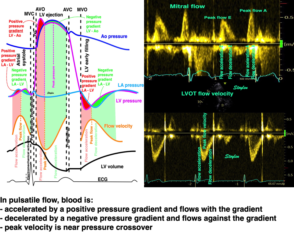
This can also be illustrated by the intraventricular pressure gradients:
This is due to the blood being accelerated to ejection velocity, meaning that the inertia will cause it to flow for a time even as pressure drops.This means that myocytes are still shortening as well, despite tension release as volume decreases due to continuing ejection. Also, any imaging modality will show continuing systolic deformation (i e longitudinal and circulferential shortening, volume decrease and wall thickening), despite myocyte relaxation, all the way to end ejection.
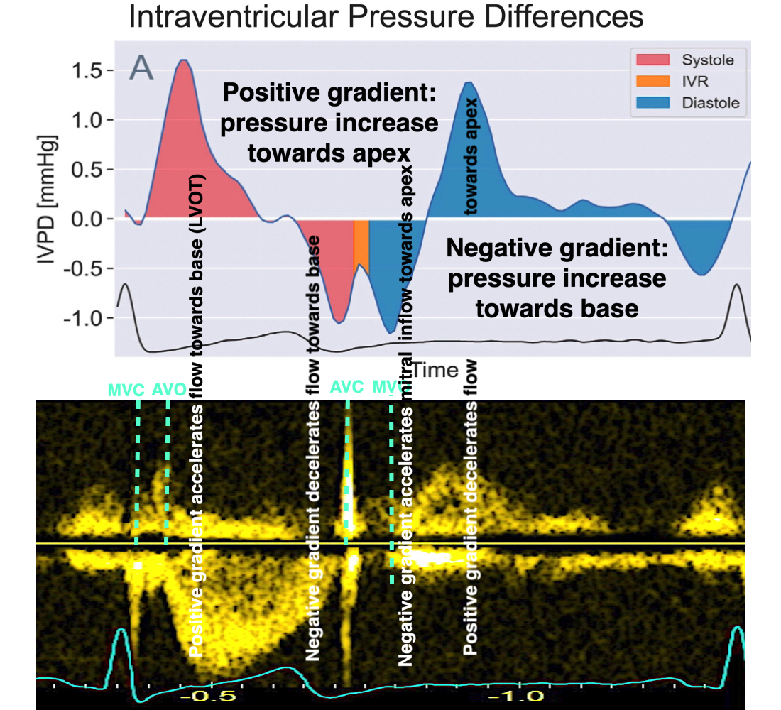
Pressure gradients derived from flow velocities. There is a positive pressure gradient during the fist part of ejection, accelerating blood towards the LVOT. The peak gradient is early, then declining with the interaction with the Aorta. At the final part of ejection, pressure gradient is negative, meaning that blood flow 1: is inertia driven, and 2: decelerates.
Myocardial relaxation is thus the force restraining the recoil (restoring forces).
Thanks to Ole-Andreas Breithardt for valuable language inputs.
This is summed up in the following figure:
It has been assumed that the first negative spike in tissue velocities after ejection was due to isovolumic relaxation, basing it on the erroneous assumption that there is elongation during IVR. This negative event can also be seen in colour M-modes of tissue Doppler, both in the mitral ring and the mitral leaflet. However, already Wiggers showed that the event relating to the closure of the aortic valve was a relaxation preceding the IVR, and he termed it proto diastole (147).
The peak negative dP/dt, is the transition point from convex to concave point . This transition should be no earlier than AVC. It has been seen to be close to the AVC (148), and has been suggested as a marker of aortic valve closure in pressure tracings, so some studies used this, but it seems that this also places the AVC reference a bit early. That study, however, used correlation between end of aortic flow and pressure traces, with no attempt to calculate bias or significance of bias.
In an early study of high framerate (149) we noticed the initial midwall elongation in the septum by strain rate, bfore the AVC. Thus, the negative spike in velocities corresponds to a protodiastolic elongation seen by strain rate.
|
|
Colour strain rate M-mode from the septum of a normal subject. It is evident that there is an elongation in mid septum, resulting in initial negative velocities in mid and basal septum before closure of the aortic valve. Notice also how the initial elongation of the mid septum occurs before the closure of the aortic valve, i.e. the initial negative velocities in the basal and mid septum are protodiastolic. | Colour TVI and SRI derived from the same recording, showing that the midwall septal elongation and the basal downward velocities are corresponding. The difference in locartion is a tethering effect. |
The basal downward motion of the septal mitral ring is also demonstrable in both M-mode, Colour TVI M-mode and spectral Doppler (72):
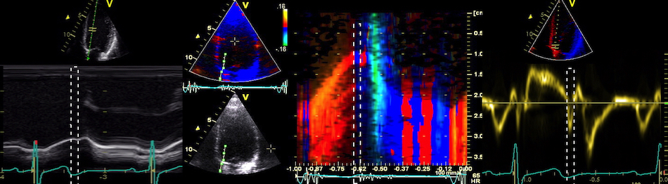
Left, M-mode of the septal mitral ring, showing a downward motion of short duration, marked by the white dashed rectangle, which is interrupted. Middle: This becomes far more evident in colour TDI M-mode, in this case where the AVC is also documented by phono. The downward motion is evident in spectral Doppler as negative velocities, that are abruptly interrupted as well.
Using first phono that was calibrated by Doppler, we were able to show that the observation by strain rate imaging was actually true. AVC was in fact at the end of the negative spike, where velocities crossed back from negative to positive, i. e. corresponding to the "notch" in the mitral ring motion (150). Although for practical purposes, the automated algorithm identifies the point of maximum acceleration, which is very close. Later we used a scanner that was modified to acquire B-mode and tissue Doppler alternating in an 1:1 pattern, and in narrow sector of the septum giving a frame rate of close to 150, imaging both the base of the septum and the aortic valve at the same time in 5-chamber and long axis views. Here, the actual closure of the AVC could be identified with a temporal resolution of about 7 ms. The study confirmed the previous findings (151), and, repeating the study in infarction patients and in high frame rate during stress echo, showed the finding to hold true (152) also outside the normal range.
The location of the AVC in relation to tissue Doppler can be easily demonstrated by the method of transferring the opening and closing events from Doppler recordings to the worksheet of analysis software, to be used in other quantitative analysis (72).
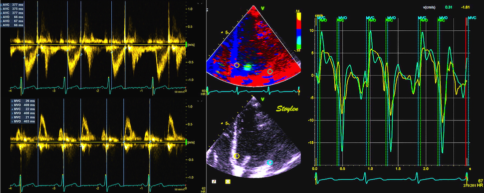
Recordings from LVOT (top left) and mitral annulus (bottom left ) with closing and opening of aortic and mitral valves marked and measured. The analysis software has then transferred the mean values for events to the tissue Doppler analysis , and the basal post ejection spike can be consistently seen before AVC, but is mainly evident in the septum.
However, this is slightly less accurate as events are transferred from separate recordings (different cycles) and thus are vulnerable to heart rate variability. But using this method, we showed that the post ejection spike was mostly located in the septum:
The negative post ejection spike thus is an onset of lenthening, that is interrupted by the AVC itself, as demonstrated shortly afterwards in an animal experiment, that stening of the aortic valve obliterated the post ejection spike itself (117).
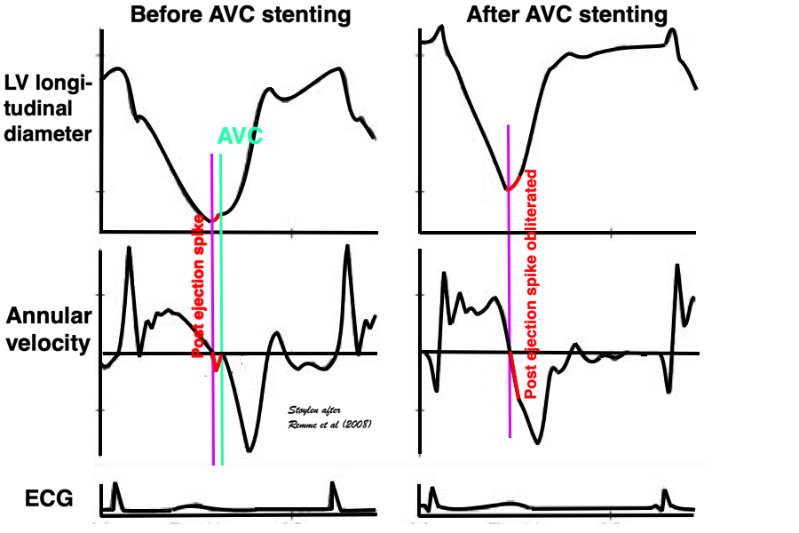
Animal experiment, showing that at minimum LV length, the ventricle starts to elongate, (negative velocity), and then the elongation stops abruptly at AVC (analoguous with the mitral ring motion), resulting cutting off the negative velocity into a spike. Stenting the AVC, results in the elongation continuing smoothly i to the filling phase, without the stop caused by AVC, and hence, the post ejection spike also being obliterated.
Thus, it is the closure ov the aortic valve that stops the initial lengthening, essentially creating the post ejection spike, and AVC is at the end of this spike. The assumption that the post ejection spike was IVR, and that AVC was at the start of this, was unfounded and erroneous.
|
|
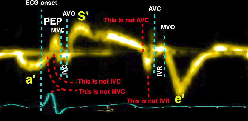
The post ejection spike corresonds to a small protodiastolic volume expansion (1.4% of EDV) before AVC (117), and can also be demonstrated by mitral ring motion (72):
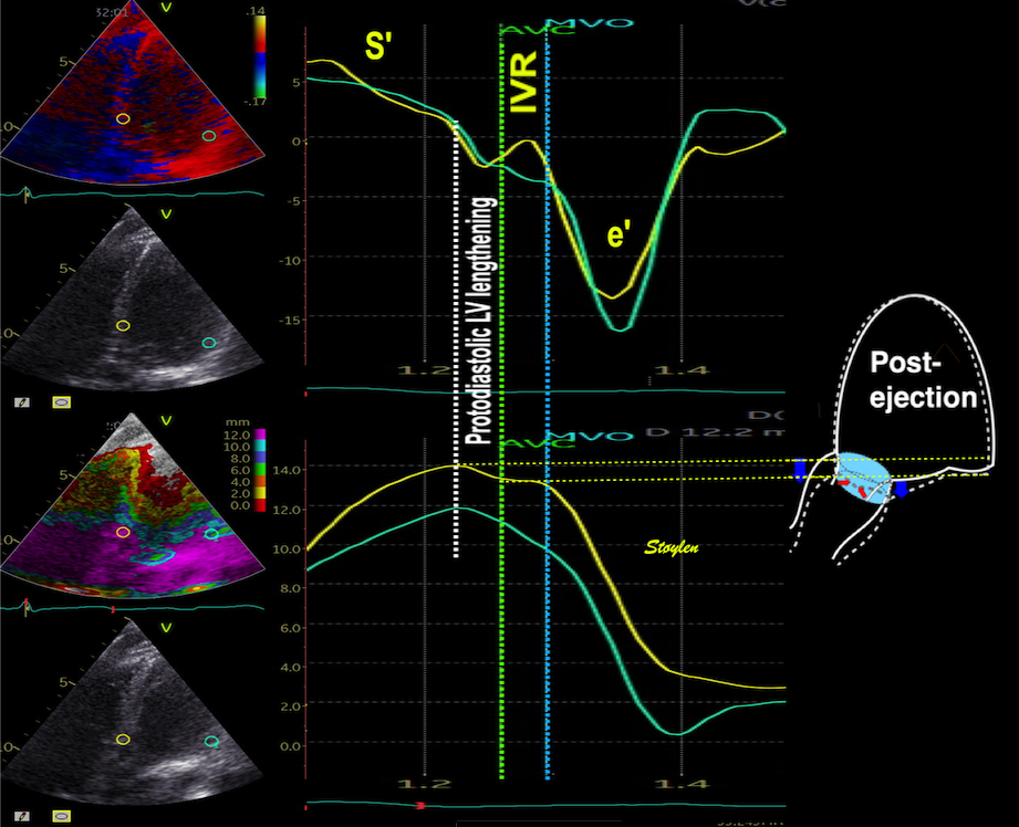
Zoomed image of the end ejection period, showing the longitudinal displacement that adds volume to the LV, the moving aortic annulus will engulf a small blood volume, not due to flow but to the annulus displacement itself.
However, in our study, the post ejection spike was only visible in some of the lateral walls, while it was evident in septum of all, but the end of the post ejection spike coincided with AVC only in the septum (72).

Post ejection spike seems to be most pronounced in the septum, both seen with ring velocity or wall strain rate.
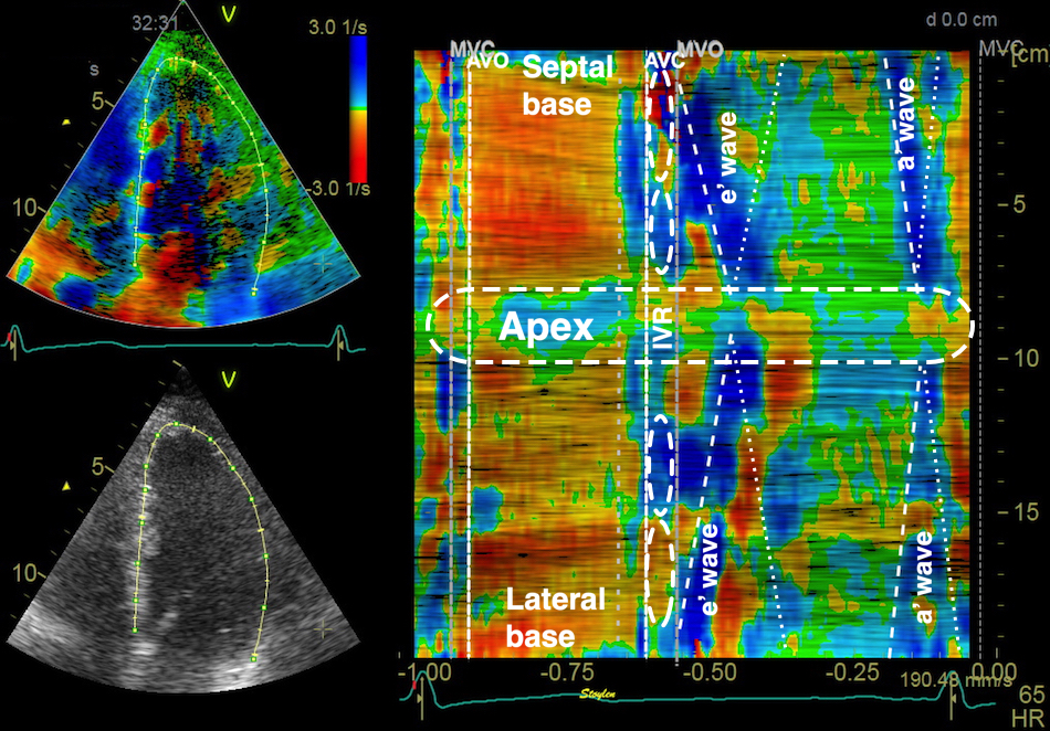
Curved M-mode showing the protodiastolic deformation before AVC, predominantly in the septum (valve motions transferred from Doppler.
The lengthening seems to be more pronounced in the septum, possibly because the open aortic valve offers less resistance to motion than the closed mitral valve to motion against the blood in the atrium.
|
|
Proposed mechanism for the aortic closure. During ejection the ventricle can be seen to shorten, and there is ejection (arrow), keeping the cusps open. Ejection is decreasing towards the end of the ejection period, as shown by the decreasing length of the arrow. At end ejection, there is no flow, and the relaxation that started during ejection as a reduction in tension, leads to a slight elongation (blue arrows). The aortic cusps then are closed due to the valve motion in the now stationary blood column, similar to what happens if a scoop is put into the water (opening forward) from a boat that is moving forward. In this case, the motion of the cusps are mainly lateral, i.e. towards the middle, and thus may be greater than the longitudinal displacement of the annulus. With the closed mitral valve, little motion is to be expected in the lateral part of the ventricle. | Volume increase due to proto diastolic lengthening. This volume increase is also evident from displacement and strain traces. This volume increase is not due to flow, but the fact that the aortic annulus includes part of the blood volume by , sliding along a stationary column of blood that then is "ventricularised", illustrated by the light blue cylinder in the image above. |

Skewed M-mode through the septum, the aortic valve and the aortic ring (which, of course is part of the AV-plane. The M-mode demonstrates the duration of the aortic closure, the onset coinciding with the peak apical displacement of the AV-plane, the closure time being the time of the post ejection elongation and hence, the protodiastole, while the end of the AVC coincides with the notch in the ring motion. The cyan line indicates the time point of the onset of the LV expansion, i.e. the end of IVC.
Thus, the AVC causes the end of the protodiastolic negative spike in the septum.
Using ultra high frame rate tissue Doppler, however, we have been able to show that the AVC event is earliest in the base, and then propagates as a mechanical event through the septum with a propagation velocity around 5 m/s, corresponding to the propagation velocity of a shear wave in similar tissue (153, 154).
|
|
Propagation of mechanical wave along septum, as visualised by ultra high frame rate TDI. The wave is identified by the peak positive acceleration in each point, showing this to be earliest in the base, lowest near the apex. The orange frame shows the velocity curves, the blue frame the acceleration curves. Image courtesy of Svein Arne Aase | The propagation velocity can be measured by colour M-mode. In this case, positive acceleration is shown in red, negative acceleration in blue. Left are the relation of acceleration visualisation in colour M-mode to the heart cycle, right an magnification of the end ejection, illustrating how propagation velocity can be measured, in the same way as strain rate propagation. |
This propagation has been demonstrated earlier (155), but not with commercial equipment.
It has been suggested that this is a marker of myocardial stiffness, as shear waves move faster in stiffer media, and thus might be a marker for fibrosis.
However, looking at the physiology of AVC propagation velocity, there are confounders galore, so taking it as a marker of fibrosis, is premature, to put it mildly. Although stiffness due to fibrosis may affect (increase) MW velocity, during a dynamic situation part of the heart cycle, many other processes which are affected by disease will do the same. Galloping after one physiological factor with new equipment is immature.
The isovolumic relaxation period is defined at the time from aortic valve closure to mitral valve opening, i.e. the period when there is no ejection or inflow to the ventricle. Thus, there can be no overall volume change, and no flow through the orifices.
Thus what happens is only tension devolution. However, most of the systolic tension devolves during IVR.
In conventional physiology the IVR is described as a pure, uniform relaxation, described by the relaxation constant, which is the constant for the pressure decline during IVRT, the tau.
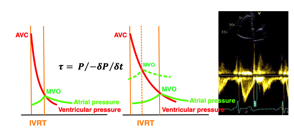
Illustration of the tau. Assuming auniform pressure decline during iVR, the tau describes the rate of relaxation. As the IVRT lasts from AVC to MVO, a cruder measure of this is the duration of the IVR., as seen to the left. With slower relaxation (reduced tau), the IVRT will be prolonged as seen in the middle. However, if the LA pressure increases in response to the decreased relaxation, this will shorten the interval between AVC and MVO again (dotted lines middle figure). The IVRT is easily measured from the AVC click to the onset of mitral flow.
So, the IVR is the period of most relaxation, (meaning tension devolution) as can be seen from the pressure curves. During IVR, there is no ventricular volume change, and thus no global devormation, volume change or flow.
However, this doesn't take into consideration intraventricular volume shifts and flow.The gold standard for defining the IVR is the valve clicks and start of flow:
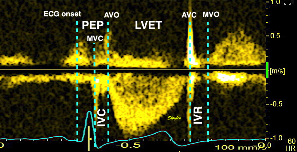
Modern software is able to transfer the timing obtained by Doppler to custom TVI analysis software;
Valve closures by valve clicks, and openings by onset of Doppler flow, to the right transferred to the analysis window for tissue Doppler to the left. Relations between timing of tissue Doppler motions and valve motions are typical. Isovolumic relaxation period (IVR), is the period from aortic valve closure (AVC) to mitral valve opening (MVO). In a Doppler flow recording with the sample volume between the aortiv and mitral valves, this is easily seen by the valve click of AVC to the start of mitral inflow.
During the IVR, there is a rapid pressure drop. The pressure curve is sigmoid, with a transition from convex curve during last part of ejection, to a concave curve at the start of mitral inflow. The time constant of the pressure drop , the tau, is taken as a measure of diastolic function, meaning relaxation rate.However, the relaxation phase, as discussed above starts at peak ejecton pressure, continues through the iVR and included the reapid filling phase (E). During end ejection, there is fibre shortening, during IVR, there is no net deformation (but differential deformation as described below), and during the early filling there is fibre lengthening.
As discussed above, there is an elongation and volume expansion at end ejection, due to continued relaxation after the flow has stopped, but this occurs before aortic valve closure, and is thus protodiastolic. It may be the mechanism for aortic valve closure itself. After the protodiastolic elongation, there is a diastolic elongation during IVR that is most evident in the apex. This occurs before the opening of the mitral valve.
During IVR, there is elongation in the apex, and simultaneous shortening of the base (72). The elongation is probably related to the ‘untwisting’ of the apex (74, 75). The basal shortening may does not necessarily indicate active contraction, but it may be a reciprocal effect of the apical lengthening, as the volume in IVRT is constant, i.e. it's only the tension inequality that causes segmental differences.
Thus, it's dubious if the shortening in reality can be classified as "work".
Peak strain rate during IVR (s-1)
Septal | Lateral | |
Apical | 0.36 (0.61) | 0.52 (0.65) |
Basal | -1.07 (0.74) | -0.36 (0.39) |
Top: curved M-mode showing the protodiastolic deformation before AVC; lengthening ocurring mainly in the septum, as well as he isovolumic period (valve motions transferred from Doppler. During IVR, there is no net volume change, so dimension changes in one part of the ventricle has to balance against opposite changes in other parts. Here, elongation in the apex (blue) is balanced by shortening in the base. However, this may create a pressure gradient(and volume redistribution) that will shift the blood towards the apex during IVR.The same can be seen in strain rate curves (bottom), elongation in the apex (positive strain rate), shortening in the base (negative strain rate) during IVR.
Looking at the tracings, there has to be regional deformation during IVR, but no overall change in volume. This would mean that there should be expansion in the apex, but without overall volume increase, this should correspond to a decrease in volume in the base.
At the start of the IVR, the anterior motion of the closed mitral valve has initiated a small, apically directed momentum. At the same time, the ejection flow is ended. During the true IVR, from AVC to mitral valve opening (MVO), there can be no overall volume change. However, with the elongation (and hence wall thinning) in the apex, and shortening, (and hence, wall thickening) in the base, there has to be a volume shift from base to apex. This corresponds to the apically directed intraventricular flow that has been described earlier (145).
|
|
Basal shortening in the base gives wall thickening, and elongation in the apex gives wall thinning, giving a volume shift from base to apex. | This volume shift can be seen as apically directed intraventricular flow during IVRT. |
The apical flow during IVRT is present in all parts of the ventricle, as can be demonstrated both by comparing colour M-modes from septal and lateral parts of the ventricle, as well as by 2D colour flow (118).
|
|
|
Colour M-mode from the septal aspect. Apically directed flow during IVRT | 2D colour flow during IVRT. (The closed MV is evident). Apically directed flow across the whole ventricle. Image courtesy of Annichen S Daae. | Colour M-mode from the lateral aspect. Apically directed flow during IVRT |
The flow is thus not related to vortex formation, but can be taken as an indication of a base-to-apex pressure gradient.
True relaxation starts during ejection at peak pressure, but the gradient is an indication that early deformation starts in the apex. There has to be a space for the blood volume to flow into. Thus, the earliest positive deformation starts during isovolumic relaxation in the apex (146). This has been confirmed by MR (74, 75).
Thus, a momentum towards apex starts during late ejection, but contiues in the IVR, driven by the heterogeneous deformation in IVR. Because of this, there is already a momentum in the LV from base to apex before opening of the mitral valve, adding to the momentum of early filling. And the inflow doesn’t start at zero velocity, analoguous to the IVC in relation to ejection. From the derived energy plots, it can be seen that thereis kinetic energy at the start of early filling. And as the simultaneous shortening at the base and elongation of the apex has a clear physiological function, the notion that shortening during IVR is "wasted work" must be considered totally non-sensical.

Colour M.mode showing the apical flow velocity during IVR continuing into the apical flow velocity of early filling.
This momentum, however, is not part of a vortex, but is mostly uni directional, with vorticity reaching a minimum, while kinetic energy starts to increase:
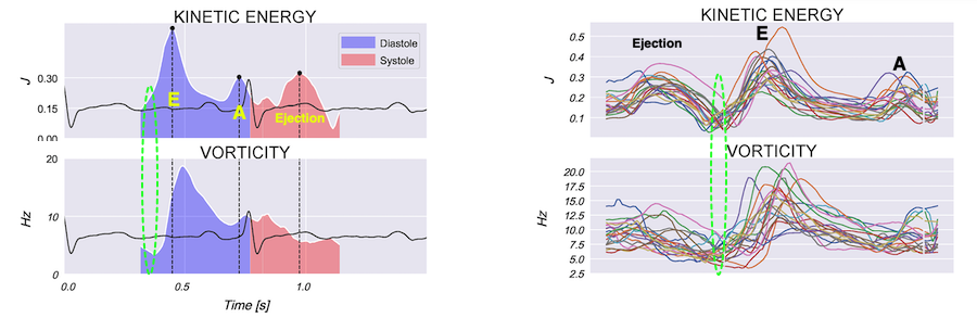
Energy and velocity plots, showing that during IVR, kinetic energy increases (as expected by the prsence of flow), while vorticity actually decreases, as expected by the unidirectional mature of the flow.
The MVO removes the ventricular volume constraint, so the ventricles can expand. Ventricular expansion and atrioventricular inflow are thus part of the same process, and thus, onset of the downwards motion of the atrioventricular plane marks the ventricular expansion, and thus the onset of flow after MVO. This process is the last part of the relaxation (tension devolution), and all of the elastic recoil.
MVO at atrioventricular pressure equalisation. Timing of MVO depends on LAP = LVP. The opening of MV removes the ventricular volume constraint, so they can expand, and releases the recoil forces, which causes volume expansion. The volume expansiojn is modified by the last part of myocyte relaxation.
Apart from identifying MVO by onset of Doppler flow, the MV is visible in all apical planes, and so MVO can be identified by M-mode, B-mode and Tissue Doppler.
M-mode of mitral plane, mitral valve and mitral flow. The protodiastolic lengthening of the LV is seen as basal motion, just after peak apical displacement, of the annulus, and the AVC is the through of the following n otch. As we see, mitral valve apical motion starts somewhat earlier than mitral flow. As flow is the rate of volume expansion, it makes sense that the start of flow actually is at the time of the onset of basal motion of the mitral ring, i.e. the lengthening of the LV.
So, as mitral annular mjotion is a marker of volume expansion, which again is related to flow; the AVC and MVO are identifiable in tissue Doppler:
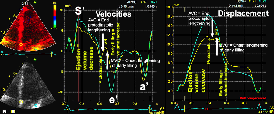
Summary of the end ejection events as seen by tissue Doppler. The protodiastolic lengthening of the septum is seen as the start of the septal negative velocity / basal ring motion, the end of protodiastole is seen as the zero crossing of the septal negative velocity / notch in the ring motion, which marks the true IVR. During IVR, there is no net volume change (ring motion), in this case the septum and lateral wall balances, and with strain this also shows as a balance between apical basal deformation as shown above. Onset of early filling is the onset of volume expansion, which again is the onset of the rapid basal velocity / motion of both walls. The volume expansion, onset of course, is the onset of flow.
Thus when the mitral valve opens, flow starts and the ventricle expands (elongates) corresponding to the downward shift in displacement of the mitral ring. However, the mitral valve opens, meaning motion of the leaflets into the ventricle, continuing the motion towards the apex. Thus the leaflets do not have the shift from positive to negative velocities. Some authors have described this anyway, but this is due to the fact that the lateral resolution in tissue Doppler is very low due to the low line density, in order to achieve a high frame rate, meaning that an M-mode line placed across the mitral leaflet close to the ring actually will be ring velocities as discussed in the measurements section. In addition, the base of the mitral leaflets will tend to follow the ring motion more than the tips. Also, the opening of the mitral valve is gradual, starting at the tips, and moving outwards towards the ring.
Looking at mitral ring traces, the logical candidate would be the moment the mitral ring starts to move away from the apex, after the "bounce" following the AVC. This would hypothetically be the time point where the ventricle starts the volume increase, seen as elongation by the mitral ring. But as this is not an abrupt mechanical event, but rater a gradual transition (an upwards convex curve in the displacement traces), this is not as easily delineated. Also , it is not necessarily present in all parts of the mitral ring (theoretically, it shouldn't, of course!).
It might be useful to do tissue doppler of the mitral valve itself, but the notion that MVO happens at the time of velocity aliasing is erroneous:
|
|
Recording of the mitral ring, (yellow), the tip of the mitral leaflets (red) and the middle of the anterior leaflet (green). Left, displacement, right velocities. The MVO is at the time of the rapid downward ring motion. Looking at the middle of the leaflet, this follows the ring motion during IVR, before starting rapid apical motion at the opening time. The mitral tip does not follow the ring motion as much, but starts rapid apical motion at the time of MVO. The leaflet reaches aliasing velocities later than the actual opening time , but as the tip moves more rapidly, this will aliase first.
The aliasing velocities of the mitral valve are later than MVO, as this marks the time when the leaflet movement (moving with the same velocity as the flow, as discussed here) reaches the aliasing velocity of the tissue Doppler, being dependent on the PRF and depth. This is also earliest at the mitral leaflet tips, as they have the most rapid motion, but still later than MVO.
Early filling start with MVO, and denotes a phase with atrioventricular inflow, which means ventricular expansion. (Flow = rate of volume increase, and is proportional with flow velocity under the assumption of a constant orifice and compliance. Looking at the pressure curve, it is obvious that myocardial relaxation in the form of tension devolution continues into early filling, but as argued above, this is a process of dissolving cross bridges, but not of restoring the original shape / length / volume.
|
|
|
Wiggers diagram. Relaxation (tension / pressure decline) starts at peak pressure, thus it is first concomitant with myocardial shortening during the last half of ejection, then with constant volume during IVR, and finally with myocardial lengthening during volume expansion. | Mitral flow velocity. The two peaks are the flow of early and late filling. The are proportional with the rate of volume expansion of the ventricle, but are functionsof the pressure gradsients. | In systole the cell can be seen to increase free calcium and simultanously shorten. In the cellular diastole, the cell can be seen to elongate, and simultaneously free calcium disappears from the cytoplasm, causing relaxation, but the calcium removal do not explain the resoring of the original length. Image courtesy of Ph.D. Tomas Stølen, cardiac exercise research group (CERG), Dept. of Circulation and Medical Imaging, Norwegian University of Science and technology. |
As most of the relaxation is already finished during IVR, the reverse deformation during early filling is due to elastic recoil. With M-mode and Doppler, however, the rate of ventricular expansion and atrial compression can be visualised.
|
|
|
Illustration of the elastic recoil. Forced deformation is shown as black arrows, recoil as red. The stiffness is related to the resistance to deformation, and the storing of elastic energy for recoil. Forced compression gives elongation during recoil, forced stretch gives shortening during recoil. | Diagram of myocardial forces and the resulting recoil forces. In systole there is longitudinal and circumferential contraction, giving forced longitudinal and transverse compression of myocytes and interstitium, as well as bending of the AV-plane. In addition, the motion of the AV-plane will stretch the large arteries. During diastole, the release will give recoil longitudinal and transverse stretch, as well as unbending of the AV-plane. In addition there must be recolil shortening of the large arteries. | Tissue velocities and motion of the AV-plane, which moves towards the apex (longitudinal compression) in systole (S), and from the apex (stretch; longitudinal recoil e'). Left is a normal ventricle, right is a patient with "delayed relaxation", which is a combination of slower relaxation, but mainly lower elastic recoil. a' is the elongation due to active atrial contraction. The delayed relaxation is evident also in the M-modes, but may be more difficult to measure, if the deflection between the diastasis and the late diastolic displacement is less sharp, and the peak early diastolic velocity (e') is a better measure. By this, we see that the peak mitral flow (E) (showing the peak rate of ventricular expansion by flow) and peak annular velocity (e') (showing the peak rate of ventricular longitudinal expansion) are related. |
Thus, the recoil is related to the length of the contraction, and the tissue elasticity, but the rate of the recoil is also related to the relaxation, in the last part of the relaxation, which modifies the recoil rate.
As shown by the M-mode, the AV-plane moves towards the apex in systole, causing longitudinal compression of both ventricles, and away from the apex in early filling and atrial systole. However, the M-mode also shows that apical motion is highest in the two lateral points, lowest in the septum, which may be construed as both a function of the wall lengths (more myocardium). This is evident as also S' is related to wall length, i.e. the regional velocity / acceleration is a function of force.
The AV-plane moves towards the apex in systole, causing longitudinal compression of both ventricles, and away from the apex in early filling and atrial systole.
|
|
| |
|
| ||
LV volume expansion starts at end of IVRT, the MVO at LA/LV pressure crossover, the volume curve showing onset of increasing LV volume. | Increasing LV volume, means LA-LV flow, as also seen by the velocities, but the peak velocities are the functions of the pressure gradients | The increasing volume is also reflected by the increasing LV length, which is seen by the downward motoion / velocity of the AV-plane. | |
Thus, the e' is the LV longitudinal recoil after MVO. This is related to LV volume expansion during early filling. As seen by the LV pressure curve above, this is the recoil after LV compression, i.e. release of passive tension built up during systole. However, this happens during the last part of decline of active tension as well.
But this is very different from a measure of relaxation rate, which is the tau.
In a bicycle study during exercise, we found that the transition from supine to sitting, presumably decreasing filling pressure, reduced both E and e', but e' more than E, so the E/e' actually increased (225). But as this was not due to increased E, it cannot be taken as an indication of increased filling pressure. In another study (171) in 18 patients with previous MI, vs. 18 healthy controls, the drop in E and e' and increase in E/e' was likewise observed.
Measure | Supine | Sitting | % | P | |
E (cm/s) | Infarct | 58 (9) | 43 (12) | - 25 | < 0.05 |
Control | 49 (12) | 39 (7) | - 20 | < 0.05 | |
e' (colour TDI, cm/s) | Infarct | 6.4 (1.4) | 3.6 (1.2) | - 43 | < 0.05 |
Control | 6.8 (2.4) | 4.4 (1.3) | - 35 | <0.05 | |
E/e' | Infarct | 9.4 (2.9) | 12.7 (4.0) | + 35 | < 0.05 |
Control | 8.0 (2.7) | 9.9 (3.2) | + 24 | < 0.05 | |
EDV (ml)41) | Infarct | 130 (31) | 103 (29) | - 21 | < 0.05 |
Control | 138 (41) | 106 (34) | - 23 | < 0.05 | |
MAPSE (mm) | Infarct | 11.2 (2.2) | 7.9 (2.5) | - 29 | < 0.05 |
Control | 12.6 (1.9) | 9.3 (2.0) | - 26 | < 0.05 | |
HR | Infarct | 59 (9) | 66 (10) | + 12 | < 0.05 |
Control | 58 (10) | 64 (8) | +10 | < 0.05 |
|
|
|
Healthy athletes, showing the transition from supine to sitting causes drop in both E and e', but with a greater drop in e', the E/e' actually increases. In this healthy group, there is no increase oin E/e' with exercise. | Healthy controls versus post MI patients shows the drop in e' and increase in E/e' with transition from supine to sitting. | Likewise there is a drop inb MAPSE from supine to sitting |
EDV and HR show a drop in LV filling pressure from supine to sitting, depite increased E/e'. But the E/e' increases due to more reduction in e' than ion E, which cannot be taken as an indication of elevated LA pressure. Secondary there is reduced SV, as shown by the reduced MAPSE. The e' is thus mainly related to volume.
Normal values for spectral tissue Doppler annular left and right ventricular diastolic velocities by age and gender from the HUNT study (16).
Left ventricle, mean of 4 walls | Right ventricle (free wall) | |||
e' (pwTDI) | a' (pwTDI) | e'(pwTDI) | a' (pwTDI) | |
Females | ||||
< 40 years | 14.6 ( 2.3) | 8.8 (1.9) | 14.7 (2.9) | 12.4 (3.5) |
40 - 60 years | 11.3 (2.4) | 10.0 (1.9) | 13.1 (2.9) | 15.0 (3.5) |
> 60 years | 8.2 (3.2) | 10.6 (1.9) | 11.0 (2.3) | 16.1 (3.1) |
All | 11.8 (3.2) | 9.7 (2.0) | 13.3 (3.0) | 14.4 (3.7) |
Males | ||||
< 40 years | 14.1 (2.7) | 9.1 (1.7) | 14.5 (2.9) | 12.3 (3.5) |
40 - 60 years | 10.7 (2.3) | 10.4 (1.6) | 12.5 (3.2) | 14.3 (3.7) |
> 60 years | 8.2 (1.9) | 11.1 (1.6) | 11.0 (3.0) | 15.8 (4.2) |
All | 10.8 (3.0) | 10.3 (1.7) | 12.5 (3.3) | 14.2 (3.9) |
Annular velocities by sex and age. Values are mean (SD). pwTDI: Pulsed Tissue Doppler recorded at the top of the spectrum with minimum gain. Values of e' decline with age, a' increase. Normal range is customary defined as mean ± 2 SD.
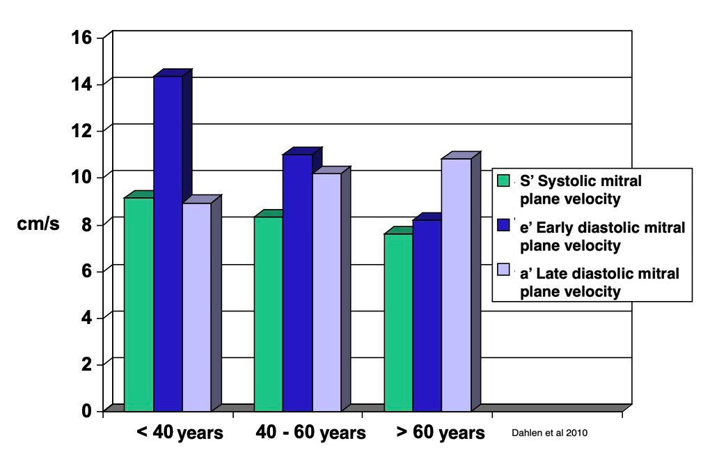
Relation between systolic and diastolic mitral annular velocities showing how the S' and e' decline with age, while a' increases.
In the HUNT3 study, we found a correlation between e' and S' (R = 0.58, p < 0.001), between e' and MAPSE, (R = 0.42, p < 0.001), but no correlation of a' with MAPSE, and only 0.18 between a' and S' (16, 156), thus showing the recoil of systolic compression to occur during early relaxation.
Thus, the recoil after the compression of myocardial contraction is basically a process during early filling, and peak early AV plane velocity, e', is a measure of ventricular diastolic function (168, 169, 170). Myocardial expansion during this phase, is due to the restoring forces, the elastic recoil of the compression generated during systole.
The recoil is elongation, thus related to myocardial expansion, more than tension, which has largely deveolved during IVR. However, there is still some tension,
length, and thus comes into play during this phase, and is due to elastic recoil of the myocytes themselves, the interstitium, the AV-plane and the large arteries.AV-plane motion, on the other hand, is more related to the volumetric end result of the AV-plane motion during the early relaxation, although the relation to filling pressure is unclear.
As for systole, the difference between walls necessitates that the global e' must be a mean of more sites, but the mean of septal/lateral, and of four walls are close.
The e' thus is a correlate of early diastolic filling volume.
Do you
think e' is the prime mover for early LV filling, & ![]() E/e' with
E/e' with ![]() LA pressure
is due to this, think again! Mitral annular motion and velocity
measure
LA pressure
is due to this, think again! Mitral annular motion and velocity
measure ![]() /
/![]() LV length, hence related to
LV length, hence related to ![]() /
/![]() volume
(inflow/outflow), not tension/pressure.
volume
(inflow/outflow), not tension/pressure.
Age | Septal | Lateral | Anterior | Inferior | LV, mean of sep&lat | LV, mean of 4 walls |
Females | ||||||
< 40 years | 12.5 (2.3) | 16.1 (2.9) | 15.1 (3.1) | 14.5 (2.8) | 14.3 (2.3) | 14.6 2.3) |
40 - 60 years | 10.1 (2.4) | 12.4 (2.8) | 11.5 (2.9) | 11.3 (2.7) | 11.3 (2.4) | 11.3 (2.4) |
> 60 years | 7.6 (2.0) | 8.9 (2.5) | 8.1 (2.3) | 8.2 (2.4) | 8.3 (2.1) | 8.2 (2.1) |
All | 10.4 (2.9) | 12.9 (3.8) | 12.1 (3.8) | 11.7 (3.5) | 11.7 (3.1) | 11.8 (3.2) |
Males | ||||||
< 40 years | 12.3 (2.7) | 15.7 (3.4) | 14.6 (3.2) | 14.1 (3.3) | 14.0 (2.7) | 14.1 (2.7) |
40 - 60 years | 9.3 (2.3) | 11.9 (2.8) | 11.0 (2.7) | 10.5 (2.8) | 10.6 (2.3) | 10.7 (2.3) |
> 60 years | 7.5 (2.0) | 9.1 (2.5) | 8.2 (2.3) | 8.1 (2.4) | 8.3 (2.0) | 8.2 (1.9) |
All | 9.4 (2.8) | 12.0 (3.6) | 11.0 (3.5) | 10.7 (3.5) | 10.7 (3.0) | 10.8 (3.0) |
Total | 9.9 (2.9) | 12.5 (3.7) | 11.5 (3.7) | 11.2 (3.5) | 11.2 (3.1) | 11.3 (3.2) |
Annular velocities by wall, sex and age. Values are mean (SD). Pulsed Tissue Doppler recorded at the top of the spectrum with minimum gain, differences between sex and age were significant; all P < .001.
So, the highest LV e' was lateral, the lowest septal. For global e', the mean of the two walls were 11.2, the mean of 3 walls 11.3 cm/s. The difference between the two means was significan (p<0.001), but as for S', totally uninteresting.
Looking at a', (which is not a function of recoil, but of atrial contraction, the highest a' was inferior, the lowest lateral, and the mean of lateral/septal was 9.7 cm/s, the mean of four was 10.0, difference was again significant (p< 0.001)
Regional systolic and diastolic velocities from the HUNT study are shown here:

The regional distribution of e' is the same as S', confirming that the recoil and unbending of the AV plane occurs during the early filling phase.
Looking at a', (which is not a function of recoil, but of atrial contraction, the highest a' was inferior, the lowest lateral, and the mean of lateral/septal was 9.7 cm/s, the mean of four was 10.0, difference was again significant (p< 0.001)
Myocardial expansion during this phase, is due to the restoring forces, recoil from the compression in systolegenerated during systole. The expansion is related to length, and thus comes into play during this phase, and is due to elastic recoil of the myocytes themselves, the interstitium, the AV-plane and the large arteries. As long as both valves are closed, the volume is locked, and the over all myocyte length isw locked as well. MVO unlocks myocyte length, and allows elastic recoil, seen by the e’. The e’ correlates both with S’ and MAPSE, showing the relation between compression and recoil, but the recoil depends on the unlocking of the volume.
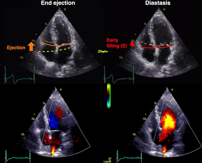
During ejection, there is longitudinal compression of the LV. The recoil is released at MVO, when inflow allows expansion, and thus myocyte lengthening.
This releases recoil:

Recoil force (red) after myocardial compression (orange), can be compared to a spring.
The reverse AV-plane motion, as well as the unbending during early filling contributes to the ventricular filling. Firstly, as the AV plane moves basally, part of the end systolic atrial volume will be engulfed by the open AV orifices, without any flow, simply because the volumes shift location from atria to ventricles. In addition, the transverse expansion (which is the recoil from circumferential shortening, as well as the unbending of the AV-plane will increase the width, and the part of the mitral and tricuspidal rings will compress the atrial volumes. This generates an atrioventricular flow during early filling.
|
|
During early filling there is recoil of the AV-plane, but only partly back to the end diastolic position, causing ventricularisation of part of the atrialised volume behind the compressed AV-plane (light red). This effect do not generate flow. | The unbending of the AV-plane will cause an additional reduction of the atrial volume (violet), causing pressure rise (the V-wave), and part of atrioventricular early flow. |
However, the AV-plane motion, can be assumed to be proportional to the volume of the early filling, as the systolic AV-plane motion is proportional to the stroke volume.
|
|
|
Analoguous with systolic strain rate, peak rate of volume increase is reflected in both early diastolic velocity and strain rate.
The apex being nearly stationary, the global diastolic strain rate (of a wall or the whole ventricle), equals the normalised, inverse value of the matching (wall or the whole ventricle) annular velocity: the annular velocity corresponds fairly closely to the wall strain rate (23).
|
|
As we see, apical velocity is close to zero, in diastole as well as systole. | Thus, the diastolic strain rate for the whole wall can be seen approximated by the basal velocity normalised for the wall length. |
But while peak systolic velocity and strain rate are simultaneous, both being the correlates for a global event, the peak rate of volume reduction, this is not the case for diastolic filling.
Looking at tissue motion from the start of early filling,
|
|
The M-mode demonstrates the duration of the aortic closure during protodiastole. The cyan line indicates the time point of the onset of the LV expansion, i.e. the end of IVC. | Tissue M-mode from the septum, showing the protodiastolic dip, the IVR interval, and the onset of basal tissue motion at the base, with a time delay from base to apex of the initiation of downward motioning the filling phase. |
Thus the onset of deformation (and volume expansion) in the early filling phase starts at be base, and is not simultaneous through the wall.
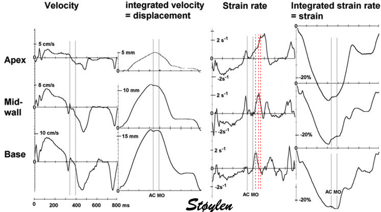
The diagram shows that the different levels has peak strain rate at different times, delayed from base to apex.
Thus, the peak strain rate of early (and late) filling, are non-simultaneous, with peaks increasingly delayed from base to apex:
This means that:
Looking at velocities at start of early filling, there is a delay in startup from base to apex, while the e' wave seems to end at the same time. This is visible both in the curves, and colour M-mode. In strain rate, however, the elongation can be seen as a wave propagating from base to apex (77).
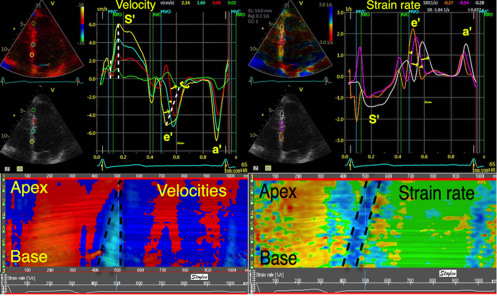
Left, velocities. The velocities of the e' sho0w a progressive delay of both start and peak from base to apex, while the ends are simultaneous. This is evident also from the triangular shape of the e' wave in the CAMM below left. In strain rate, the e' peaks show delay delay of both start, peak and end, from base to apex, as also seen by the elongation wave propagating from base to apex in the CAMM below right.
Thus, the recoil is not a single liberation of events, but an ordered sequence, liberationg recoil in a spatial sequence.

The elastic recoil, however, is not a si,multaneous even, but an ordered sequence from base to apex as shown by strain rate.
How can this be explained?
Firstly, the motion has to start at the base, as the direction of the motion is basal. As the apex is fixed (against the chest wall and pericardium, motion has to go in the basal direction (away from the apex. Compare with a row of standing cars, if the row shall start to move, motion has to start with the foremost.

Colouring the cars acquiring velocity in blue, we see the start of the wave in front, adding one car at a time till all have the same velocity, and thus are blue. Colouring only the cars with DIFFERENT velocity, we show the interval where distance increases, i.e. where the row deforms (stretches). It shows the difference between deformation and motion, and illustrates that the diastolic deformation is a discrete event, propagating in a wave.
Thus, the propagation of the filling wave is another measure of diastolic function:

A: In this animation, the two autos where distance increases (the one starting up, and the next, standing still) are coloured cyan to visualise the segment with positive strain (lengthening). The time delay of initiation of motion from one element to the next, creates a wave of increasing distance between the elements that propagates backwards, while the autos move forward. This is analogous to the elongation waves from base to apex during the filling phase. Below this is illustrated as an M-mode.

B: In this animation, the autos have reduced velocity after start, compared to the one in A. This can be seen by the decreased distance between the moving cars. The propagation wave becomes slower as the cars drive slower. This is analogous to a reduced rate of local relaxation (lower early diastolic strain rate. M-mode below.
C: In this animation, the autos move with the same velocity as in B, once they have already started, but the time between the start of each auto have increased. This also shows up as increased distance between the moving cars, but here the increased distance is due to delay in starting, not a decrease in velocity, compared to B. This is evident if looking at the distance the the cars have moved from one frame to the next. This also leads to a slower propagation of the elongation wave, and this effect is analogous with reduced propagation per se, even if the local relaxation rate is unchanged. M-mode below
|
|
|
|
Showing the cars in an M-mode plot, but Tilting the M-modes 90°, the motion is downwards and the elongation wave propagates upwards, as in a conventional M-mode of a myocardial wall that is shown to the left. The red line shows the elongation propagation upwards, , the black line shows the motion of the front of the car queue downwards. This is situation A. | Situation B; the cars have reduced velocity, the M-mode shows reduced slope (velocity) both of the strain rate propagation and the motion of the car front. | Situation C: The cars have the same velocity as in A, but the start of each car is delayed relative to the car in front. This can be seen to reduce both the downward velocity of the car front, and the upward propagation of the strain rat6e. | Diastolic strain rate propagation velocity is the slope of the elongation wave. |
Going back to the LV, the strain rate propagation is the propagation of the elongation and thinning wave going from base to apex, while the velocity is the continuous motion of the base, and successively the wall, away from the base.

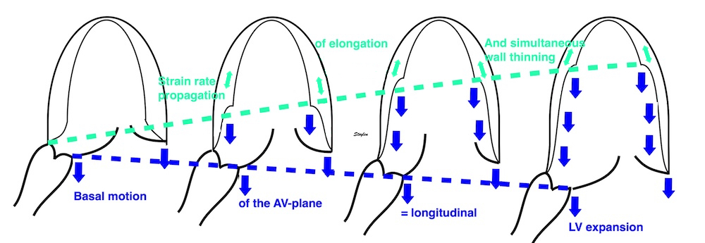
Elongation starts at the base, where the myocardium closest to the mitral ring is first that is free to move basally. This basal motion continues through the full early filling phase, and new myocardial tissue is added to the motion. The simultaneous elongation and thinning of the wall proceeds towards the apex as a discrete wave of cavity expansion, but the elongated and thinned myocardium will still be moving.
The similarity to the early filling phase is evident.
Secondly: the longitudinal shortening of the LV also stretches the large arteries, that are attatched to the center of the AV-plane, which then will recoil by shortening:
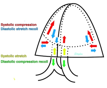
Diagram of myocardial forces and the resulting recoil forces. In systole there is longitudinal and circumferential contraction, giving forced longitudinal and transverse compression of myocytes and interstitium, as well as bending of the AV-plane. In addition, the motion of the AV-plane will stretch the large arteries. During diastole, the release will give recoil longitudinal and transverse stretch, as well as unbending of the AV-plane. In addition there must be recolil shortening of the large arteries.
The importance of this mechanism is uncertain.
It is important to realise that this propagation of a deformation (elongation) wave does not mean that the relaxation propagates from base to apex. The diastolic function of the myocytes is a local event, depending on the rate of relaxation (tension decline) due to the rate of inactivation of myocardial cross bridges, which again is related to the rate of removal of calcium from the cytoplasm as discussed above. In addition there is the elastic recoil, which is both inherent to each myocyte and to the heart in total. Thus it is deformation that starts in the base, not relaxation.
We can se that the both the early and late filling are propagatoing from base to apex, and the mechanism for that is the same for both, as discussed here. However, the propagation velocity differs, being higher in the a' wave than the e' wave (77).
e' (cm/s) | a' (cm/s) | PVSe' (cm/s) | PVSa' (cm/s) |
13.1 (2.8) | 10.2 (1.8) | 60 (12.9) | 94.0 (22.1) |
As the LV myocardium is under tension, although relaxing during the e', but being completely relaxed during the a' (at least in normal EDV), this is not surprising.
The strain rate propagation is reduced in reduced diastolic function (77). However, this is not a "new" finding, but relates to the finding of reduced e' in tissue Doppler.
|
|
Relation between diastolic strain rate propagation of the E-wave and the peak early diastolic velocity of the annulus. If the wave propagates slower, the resulting velocity wave of the annulus will be broader and lower . | In reduced diastolic function as shown here to the right, there is a lower peak diastolic annular velocity as well as a reduced early magnitude of motion of the mitral ring. |
Strain rate propagation is thus a global measure that relates geometrically to the peak e' in tissue Doppler.
Thus, there is a geometric relation between strain rate propagation and e', which is both theoretically and empirically probable.
In a comparison study between normals and hypertensive patients with reduced diastolic function (165):
N | Age | EF (%) | S'(cm/s) | HR | LVDd (mm) | E (cm/s) | Dec-t (ms) | IVR (ms) | A (cm/s) | e' (cm/s | a' (cm/s) | PVSe' (cm/s) | PVSa' (cm/s) | |
Controls | 28 | 40 (14) | 56(6) | 9.5 (1.6) | 63 (11) | 57(5) | 74 (13) | 183 (32) | 77 (15) | 53 (14) | 13.1 (2.8) | 10.2 (1.8) | 60 (12.9) | 94.0 (22.1) |
Patients | 26 | 65 (11) | 55(6) | 7.0 (1.1) | 61 (14) | 53(11) | 70 (20) | 252 (48) | 103 (19) | 74 (19) | 8.2 (1.5) | 11.0 (1.8) | 31.6 (9.3) | 72.0 (16.2) |
P: | <0.001 | NS | <0.001 | NS | NS | NS | <0.001 | <0.001 | <0.001 | <0.001 | NS | <0.001 | <0.001 |
Interestingly, there is a small reduction in systolic function as well (by S'), and the reduced diastolic function is moderate, although there is reduced E/A ratio both in Doppler (due to increased A) and dec-t, and in tissue Doppler (due to reduced e'). The lower diastolic function is most evident in e', but also in the propagation velocity of early diastolic strain rate, as they are interconneted as shown in the figures above.
However, using strain and strain rate, the diastole can be seen to be far more complex, showing a sequence of events that are different, and with different timing in the different segments. Thus is seen due to the better spatial resolution, as deformation imaging eliminates the effects of the tethering of the base to the more apical parts. In addition, these events interact, to result in the simpler pattern seen in motion traces, and the main finding is that there are more than one peak in each of the two phases of e' and a'.
Curved M-mode showing the full M-mode from basal septum through the apex to the basal lateral wall. The isovolumic phases with apical lengthening and basal shortening is seen, as well as the propagation of the elongation waves both in early filling phase and during atrial systole, which also shows a propagation from base to apex, but with a higher propagation velocity. In addition, the elongation waves can be seen to either cross or return from the apex towards the base, but far weaker. This can also be seen above, as the basal strain rate are double peaked.
|
|
CAMM and curves from the septum, showing the complexity of the diastolic strain rate with the different peaks resulting from both elongation pre AVC, apical elongation during IVR, elongation during early and late filling, and return waves from apex, resulting in double waves in the midwall and base. | Curved M-mode through the whole wall, showing how the elongation waves look contiguous across the apex. |
The clinical importance of this finding, however, is uncertain.
And the whole heart cycle can also be visualised by the motion and deformation measures in a combined diagram analoguous to the Wiggers diagram as seen below:

The heart cycle visualized by motion and deformation measures , all from tissue Doppler of the same cine loop. Valve openings and closures are taken from Doppler flow registrations, and transferred by the software to the actual heart cycle.
|
The recoil of the AV-plane is shown by the e' wave, the velocity of the longitudinal expansion of the ventricles. |
Thus, the difference between the annulus diameter and and the ring diameter is consistent with the presence of transmitral E and A flow (174).
The AV-plane moves towards the base in early diastole, causing longitudinal expansion of both ventricles, but als a concomityant compression of the atriaand the difference of atrial and ring diameter, causes the flow of blood from atria to ventricles.
This will cause the pressure to drop less in the atria, compared to the ventricles, driving flow.
So there is concomitant ventricular pressure drop (negative dP) and volume expansion (positive dV) so the compliance (dV / dP) is negative. Flow (and volume expansion) are driven by the atrioventricular pressure difference).
AV-plane motion, mitral valve motion and transmitral flow.
Traditionally evaluation of left ventricular diastolic function has been by mitral flow (158). As flow is related to pressure, the typical combination has been pressure - flow diagrams, as shown below:
|
|
|
|
Relation between mitral flow indices and pressure in the normal situation. Mitral flow (orange curve) is dependent on the pressure gradients between the left ventricle and the atrium, created by left ventricular relaxation and recoil. The decline in pressure gradient during IVRT ( = relaxation constant tau) after AVC determines the length of the isovolumic relaxation time. The decline in the pressure difference between atrium and ventricle as the ventricular pressure increases, determines the accceleration time. This again is dependent on the relaxation rate, as the active relaxation, creating a quick recoil and pressure drop in the ventricle, a high gradient and a short acceleration time. Atrial pressure, increasing somewhat slower due to filling, reverses the pressure gradient, whoich decelerates mitral inflow. Thus deceleration time is dependent LV recoil /relaxation. Atrial pressure increases during atrial systole, forcing blood to flow again in the A wave. | Slower relaxation leads to a decrease in the tau, and thus a longer IVRT before the mitral valve opens; Increased IVRT. In addition, the slower relaxation leads to a slower and smallerdrop in LV pressure, leading to a reduced reduced peak E flow, and a slower rise in atrial pressure, and thus a longer deceleration time. The lower filling volume leads to a higher atrial volume at the start of atrial contraction, and thus a higher atrial stroke volume (perhaps by the Frank-Starling mechanism), and a higher A- wave. The E/A ratio is reversed. |
Normal values for the mitral flow indices from the HUNT study (16).
Mitral E | Mitral A | E/A | DT | IVRT | |
Females | |||||
<40 years, N=208, mean (SD) | 80 (16) | 48 (15) | 1.85 (0.76) | 212 (55) | 85 (16) |
40-60 years, N=336, mean (SD) | 74 (15) | 59 (15) | 1.32 (0.40) | 220 (66) | 95 (20) |
>60 years, N=119, mean (SD) | 69 (16) | 75 (18) | 0.96 (0.32) | 244 (79) | 105 (23) |
All, N=663, mean (SD) | 75 (16) | 58 (18) | 1.42 (0.62) | 218 (66) | 93 (21) |
Males | |||||
<40 years, N=126, mean (SD) | 75 (15) | 44 (14) | 1.86 (0.64) | 217 (65) | 91 (17) |
40-60 years, N=327, mean (SD) | 64 (15) | 52 (14) | 1.30 (0.42) | 232 (81) | 100 (21) |
>60 years, N=150, mean (SD) | 61 (14) | 65 (18) | 0.99 (0.34) | 269 (97) | 118 (29) |
All, N=603, mean (SD) | 66 (15) | 54 (17) | 1.34 (0.54) | 238 (85) | 103 (24) |
Total | 70 (16) | 56 (18) | 1.38 (0.58) | 228 (76) | 98 (23) |
Both IVRT, E and Dec-t decline normally with age, while E/A increases.
|
|
|
Normal mitral flow inh various aged persons, left: 20 year, middle, 50 year and right 70 year. Remark the decreasing E and Dec-t, and the increasing IVRT, A and E/A ratio with increasing age.

Delayed relaxation, showing values outside the normal range.
Basically:
Length and velocity are both related to volume changes, and are the resultant of tension vs. load. Both E and e' are related to tension vs load, and e' is not the cause of early pressure changes.
Relation of pressures, flow velocity, volumes, strain rate and strain. Strain and strain rate are measures related to relative volume changes (EF), and are thus functions of tension vs. load, andn not measures of contraction ( tension) nor contractility.
But this also means:
In line with what has been described for ejection, while stationary blood is accelerated along a positive pressure gradient, flowing blood is decelerated by a negative pressure gradient. Early mitral flow has a pattern of acceleration to peak flow, and then deceleration to zero. This must be due to a reversal of the pressure gradient, with peak flow at pressure crossover.
|
|
The firgure shows the biphasic pressure gradients both during atrial systole, ejection and early filling, and how this will generate an acceleration-peak-deceleration flow velocity pattern. | Both LVOT flow, and mitral E and A flows has the påattern of staring at zero, accelerating to peak velocity, and decelerating to zero again. Peak velocity will be close to pressure crossover. |
For early and late diastole, this has been documented in experiments (264, 269, 270)
Early mitral flow velocity is a function of ventricular expansin, which is the recoil from systole, modifies by myocyte relaxation. This generates a pressure drop in the ventricle, which aspirates blood from the atrium. However, the driving force of the atrioventricular flow is the atrioventricular pressure gradient, so the atrial pressure is another comnponent deciding flow velocity:

Diastolic function diagram shown by pressure and flow traces.
A: | B: Decreased LV end diastolic compliance may be due to due to fibrosis dilation or hypervolemia, leads to a higher increase in LV pressure from the injected volume from the atrium. This leads to an earlier equilibration of LV and LA pressure, and an abbreviated A-wave, which can be seen by comparing with the duration of the reverse A wave in the pulmonary veins. Decreased LV compliance shows up first in end diastole, as this is the phase where the ventricle is at the highest volume. | C: | D: If delayed LV relaxation leads to slower LV filling, this may lead to congestion of the LA; i.e. increased LA pressure (filling pressure). This will lead to earlier MVO, despite the slower relaxation, and thus the IVRT will decrease again. Thus, the pressure gradient is higher during early filling, giving higher peak E flow. Thus the LV pressure increases faster in response to the filling from the LA, due to both the increased filling rate, slower relaxation and finally less compliant ventricle already during diastasis, and the dec-t is also reduced again. The pressure gradient in diastasis may even give flow in diastasis (an L-wave, as shown here. |
In diastolic dysfunction, ventricular filling may be impaired by the slower relaxation. This may increase atrial pressure. Increased atrial pressure reduces IVRT due to earlier mitral opening. The increased atrial pressure will also increase the peak early pressure gradient and peak early flow velocity, the E increases and the Dec-T decreases towards normal values again (158).
|
|
|
Patient with apparent normal IVRT of 88 ms | Normal Dec-t of 242 ms and E/A ratio of 0.85 | However, reducing left atrial pressure by the Valsalva manouver, demasks a delayed relaxation pattern, with Dec-t 750 ms and E/A ratio of 0.36, showing the pseudonormalisation by increased left atrial pressure. |
In advanced cases, The E/A ration becomes increased over the normal limits, and IVRT and Dec-T becomes sub normal, in the restrictive pattern:
|
|
|
|
Restrictive mitral flow in heart failure. E/A ratio: 2.45, dec-T 219 ms. See also short IVRT. | Same patient after intensive treatment with ACE inhibitor and diuretics. LA pressure is normalised, and dimitral flow now shows delayed relaxation, with longer IVRT and Dec T, and reversed E/A ratio. |
The annular plane early diastolic motion is related to LV volume increase during early filling, and thus governed by elastic recoil and the rate of relaxation. It is, however, still a mproxy of the volume change during early relaxation, not the cause of the voluyme change.
It has been suggested, nearly universally, that e' is the cause of the pressure changes, while flow is the resultant. This was based on the findings that with oncreasing atrial pressure, there was a discrepancy beween mitral flow, showing increasing E, and tissue velocity, which do not increase as much with atrial pressure, and thus there will be an increasing discrepancy between the two measures, and an increasing ratio of E/e' with increasing atrial pressure (168, 169, 170).
|
|
A: Patient < 30 with normal diastolic function. E/A > 1, Short Dec.T and IVRT, high e'. In this patient it is normal for age, but might have been severe heart failure with restrictive filling, even given the patient's age. | B: Patient about 50 years with near normal diastolic function. for age. E/A = 1, somewhat longer Dec-T and IVRT. |
|
|
C: Slightly impaired relaxation. Patient at about 70, with slightly delayed relaxation due to a history of hypertension. Prolonged IVRT, dec-T, reduced E and E/A ratio < 1. Also reduced e'. | D: Severely impaired relaxation. Patient with heart failure (and normal EF and LV EDV), but with normal filling pressure due to diuretic and ACE inhibitor treatment. Severely reuced relaxation with prolonged IVRT, dec-t, decreased E and E/A ratio <<1. Very low e'. |
|
|
E: Pseudonormalisation. Patient age 69 with history of hypertension. Mitral flow (top left) shows normal values for E, A and Dec. time, and the IVRT (top right) is also normal. Tissue Doppler (bottom) shows impaired relaxation, (E/e' about 15), indicating that the atrial pressure is elevated.This is the same patient with the Valsalva manouver above. | F: Patient with restrictive pattern (actually same patient as in C, but before treatment, and then with increased LVEDV and low EF), due to high filling pressure. Short IVRT, dec-t, high E and E/A ratio. e' still low showing that there is delayed relaxation, despite the high E and E/A. Compare with A, little difference, but taking the patient's age into consideration, it is actually evident that this is restrictive filling, even without tissue Doppler showing a low e'. |
As explained above, longitudinal motion and velocity are both related to volume changes, which are a function of tension vs. load. Thus, the idea that e' is the prime mover, and thus the cause of the pressure drop in early filling, is erroneous.
There is a peak E flow velocity / peak e' tissue velocity discrepancy in elevated filling pressure, but the cause is another:
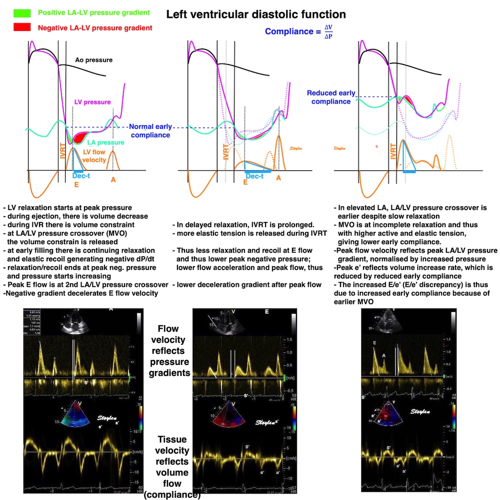
The concept that the E/e' ratio is due to the fact that e' is the cause of pressures, while flow is the result, is erroneous. The discrepancy is due to the fact that while flow velocity is related to pressure gradients, tissue velocity is related to volume flow, and thus to early compliance.
Still, the E/e' ratio has been used for assessment of atrial pressure, and documented in studies, despite resting on erroneous physiological assumptions (168, 169, 170). If both E and e' increases, the ratio remains unchanged, and the increase in flow is due to higher relaxation rate as in exercise in normals (171). However, if E increases without e' increasing simultaneously , the increase in flow must be driven by increased filling pressure instead of by relaxation as in exercise in patients with impaired relaxation reserve (171), and the increase in the E/e' ratio is related to the increase in filling (atrial) pressure. However, if E remains unchanged and e' decreases, it is not physiologically meaningful to take the increased ratio as a measure of increased filling pressure. In fact, in transition from supine to sitting the E/e' increases while filling pressure decreases (171). Thus the E/e' relates only to filling pressure when E increases.
An E/e' < 8 is considered normal, while E/e' > 15 is considered a sign of elevated LA pressure.
However, there are caveats:
Mean e' by site in the HUNT3 study
Mean | Septal | Anterior | Lateral | Inferior | |
e' (SD) cm/s | 11.3 (3.2) | 9.9 (2.9) | 11.6 (3.7) | 12.5 (3.5) | 11.2 (3.5) |
and then so must the E/e', as shown in the HUNT3 study (16).
E/e' from pwTDI according to age and site of e' measurement
Mean of four points | Mean septum-lateral | Septal | Anterior | Lateral | Inferior | |
All | 6,6 (2,1) | 6,6 (2,1) | 7,5 (2,4) | 6,6 (2,4) | 6,1 (2,2) | 6,8 (2,3) |
<40 years | 5,6 (1,3) | 5,6 (1,3) | 6,5 (1,7) | 5,4 (1,6) | 5,1 (1,3) | 5,7 (1,6) |
40-59 years | 6,5 (1,7) | 6,5 (1,8) | 7,4 (2,0) | 6,5 (2,0) | 6,0 (1,8) | 6,7 (2,0) |
>60 years | 8,2 (2,6) | 8,2 (2,7) | 9,0 (3,1) | 8,5 (3,0) | 7,6 (3,0) | 8,4 (2,9) |
It is evident that there is considerable site dependency of the E/e' as well. It is also evident that there is little difference between mean of four points versus two points, when only mean and SD are considered.
< 40 | 40 - 60 | > 60 | All | |
N | 327 | 651 | 263 | 1241 |
Mean | 5,6 (1,3) | 6,5 (1,7) | 8,2 (2,6) | 6,6 (2,1) |
As long as the peak of the E is discernible, the E/e' is meaningful, but with complete fusion, the combined flow velocity will be E+A, which is not meaningful in relation to the E/e' ratio. This point is important in three situations:
- Children have higher heart rates, and partial fusion is common at rest, and even total fusion in neonates.
- First degree AV-block may give fusion at normal resting heart rates.
- In exercise testing, the increasing heart rate leads to total fusion, usually at HR around 100. This means that for diastolic dysfunction, exercise tests are not as useful at HR > 100. In dysfunction due to ischemia at higher heart rates, however, ischemic stunning may persist for some time, while heart rate falls, and may still be useful.
It might be tempting to compare this strain rate propagation to flow propagation.
While strain rate propagation is a sharply delineated phenomenon, flow propagation may be measured in various ways:

Colour M-mode from a normal ventricle. In this image, early filling (E) can be seen as a fairly steep wave from base to apex. The propagation velocity is the slope of the column, but as seen, values varies depending on how it is measured, as the front of the column (black to colour), the front of the aliasing velocity or the main vector of the aliased velocity (which both will depend on the PRF). The black-to-colour, however may be difficult to discern from the intraventricula flow during IVR.
All measures have been used in studies (159, 160, 161, 162)
However, flow propagation as seen by colour M-mode, is not the inflow of blood, as related to the volume expansion, but the propagation of the velocity vectors.
In a normal study (163) of 12 subjects, the mean values were as follows: Black-to-colour: 55.5 cm/s (17.7), Front of aliased contour 54.8 (5.5), main aliased vector 72.1 (40.6), showing the front of the aliased contour to be the most robust, with least variability, but, dependent on the PRF setting. However, the mean aliased velocities in the inflow column are closest to the peak of inflow velocity (peak E). Peak E in the same group was 73.6 cm/s and strain rate propagation in the same group was 66.6 cm/s. In a recent normal study (118), we found peak E 82 cm/s and flow propagation velocity (by front of aliased contour to be 66 cm/s.
In both studies, thus, the peak inflow velocity was higher than the flow propagation velocity of the peak velocity vectors, but the strain rate and flow proagation corresponded fairly well, considering there are differences in measurements as shown above.

Strain rate and flow propagation. In the normal situation, the inflowing blood will fill the expanding space created by the combined elongation and wall thinning. As this starts in the base, the first (1) inflow of blood will be diverted to this filling, while the blood in the inflowing column will be substituded with later arriving blood.This process will then repeat with the next batch of blood (2), filling the cavity expansion moves towards the apex, and later arriving blood is replacing the inflow column. Thus, the flow propagation is the velocity vectors that propagate, while the blood column itself is replaced during filling..
Diastolic deformation propagates from base to apex when there is blood to fill the void that is created, unlocking the local recoil.
As inflowing blood at the flow front is diverted laterally to fill the emerging void, later parts of the inflow column moves to the front. Thus, Vp< E in healthy subjects, but Vp is similar to SRp (measurements not perfect)., in the normal subjects (163, 165), flow propagation was 55 cm/s by aliasing front, strain rate propagation 60 cm/s in the normal subject group.
This is the third explanation for the ordered sequence of the filling phase from base to apex (strain rate propagation): As the MVO initially liberates the recoil force, the inflowing blood will unlock the recoil lengthening as it fills the ventricle sequentially from base to apex. Thus, this is blood flow / myocardium deformation interaction.
flow propagation is a more complex phenomenon, consisting of both a propagation of velocity vectors, not volume propagation, and a vortex formation, that also propagates more slowly towards the apex (166, 167).
Looking at the inflow, flow propagation is obviously related to vortex formation. As the mitral orifice diameter is smaller than the LV diameter, flow must diverge as soon as it passes into the ventricle. This is also facilitated as the ventricular base moves basally at the onset of MVO.
increasing the available volume behind the mitral ring. At the start, this creates vortices on both sides of the inflow column, rotating in both directions.
Septal colour M-mode showing reversed flow towards the base starting in mid ventricle immediately after MVO (valve signal) simultaneous with the basal motion of the LVOT. | Vector flow image showing diverging flow into the LV, due to the wider ventricle, in combination with the expansion due to the basal motion of the mitral ring. The inflow is heavily aliased due to the PRF in the application, Nykvist does not correspond to the colour M-modes. Image courtesy of Annichen S Daae. | Lateral colour M-mode showing a much smaller reversal signal in the lateral aspect of the ventricle, due to the smaller volume. |
As the volume in the LVOT is far bigger, and thus increases the most by the annular plane motion, the vortex generated here will dominate, while the lateral vortex, being smaller and in the opposite direction will extinguish. It was evident from the study, both by vector flow and CMM that the LVOT vortex forms in mid ventricle, before flow has reached the apex (116).
The inflow into the LVOT during filling can be demonstrated even by pw Doppler:
Pw Doppler with sample volume in LVOT, but close enough to see the mitral inflow signals as well (E and A). In the LVOT delayed signals can be seen in the opposite direction, diverted flow from mitral inflow as the LVOT expands (ELVOT and ALVOT).
During early filling, the kinetic energy is at a peak. However, vorticity peaks slightly later during early filling, which is consistent with the formation of an early new vortex during early inflow. Images courtesy of Morten S Wigen.
Peak ELVOT was delyed on the average 116 ms compared to E in the study (116), previous authors about the same (80 - 200 ms) (164). To exclude the possibility of this being wall signals, Q-peak e' was also measured. Peak e' was shown to be 13 ms before peak E, confirming that the downwards annular motion was concomital with early filling, and thus with volume expansion, while LVOT inflow was a different event.)
Illustraton of time delays of the verious signals from the LVOT: Top: the E and ELVOT with an average delay of 116 ms. Bottom, ECG-aligned tissue Doppler from the same patient, showing near simultaneity of E and e', meaning that the ELVOT is later. In the middle, the wall filter has been reduced showing that the wall signals are tissue signals. | Illustration of the delayed inflow to the LVOT, the e' is very visible in the signal to the right, before ELVOT, and to the right with low wall filter and reduced gain from the same subject, the full TDI signal is visible. |
The timing of the ELVOT supports the notion that the flow is detected very early during inflow, and not at the apex. In the present study peak E was 82 cm/s and peak A 56 cm/s. With an average length of LV of 9 - 10 cm, this would mean that flow returning via the apex would appear in the LVOT in over 2 seconds, so the notion that the A LVOT was the E returning from the apex is erroneous.
Septal colour M-mode, showing the vortex inflow to LVOT, but at the same time, propagation of the downward flow vectors towards the apex, as the vortex expands. | While the flow reaches the apex, the velocities decrease as seen by the colours, from aliased to yellow through orange to red. The vortex created at the base, expands towards the apex at a slower rate. Image courtesy of Annichen S Daae. | Lateral colour M.mode, showing inflow velocity propagation, but also how this decelerates by time and distance toward the apex (colour intensity decreases from aliased to yellow through orange to red). Vortex propagation (expansion) propagates at a slower rate. |
As we have previously shown that the volume expansion of the LV during filling starts at the base, it actually follows logically that the early inflow must be deflected to fill the base first.
Thus, it seems to be the case that the flow front is deflected, and do not flow directly towards the apex, but rather is being substituted by later arriving blood in the forward column, so the inflow propagation is slower than the flow. At the same time, the strain rate propagation represent both elongation of the chamber and thinning of the wall (chamber expansion), and thus is also part of the changing geometry facilitating the vortex formation.
Successive stages of early filling, showing how inflow velocity decreases (colour from aliased to yellow through orange to red), as the inflow vortex at the same time expands, to fill the whole ventricle. At the end of early filling, inflow to the LVOT reverses again towards apex, creating a full vortex. Images from loop courtesy of Annichen S Daae.
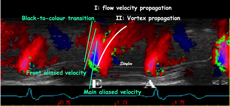
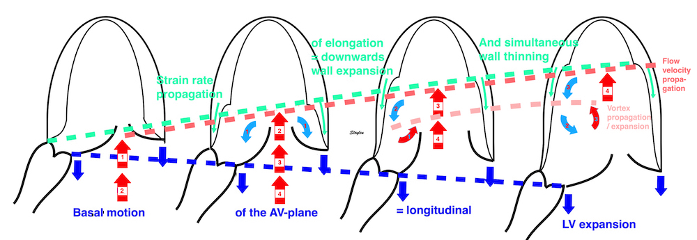
Flow propagation was originally thought to be a measure of diastolic function (159, 160, 161), but as diastolic dysfunction is more prevalent in dilated Hf, it seems that the dilated ventricles is a confounder, giving a preponderqance of vortex formation and propagation due to dilation (166, 167), which is cinfused with the proper flow propagation.
|
|
Inflow during early filling in a normal subject. The E wave can be seen as a fairly steep wave from base to apex (I), followed by a more "smeared out" wave arriving later in the apex, representing the vortex following the initial flow velocity propagation. | Inflow in a dilated ventricle ventricle of a patient with heart failure. Flow propagation is reduced, not due to the reduced propagation of velocities in the early phase, but because most of the flow propagation is vortex propagation. |
In diastolic dysfunction without dilation, however, it seems that the flow propagation velocity is actually increased (163). In the study mentioned above, a subset had flowpropagation measured, both in controls and in patients with reduced diastolic function.:
In this group, the strain rate propagation, as well as all diastolic functional measures was reduced, while the flow propagation was increased. The patients were older (mean 46 vs 64), so the effects on diastolic function was partly hypertensive, partly age dependent.
IVSd (mm) | LVIDd (mm) | EF (%) | E (cm/s) | Dec-t (ms) | IVR (ms) | E/A | e' (cm/s) | Strain rate prop (cm/s) | flow velocity prop (cm/s) | |
Controls | 7 | 57 | 57 | 74 | 191 | 73 | 1.74 | 12.8 | 66.6 | 54.8 |
Patients | 10 | 54 | 54 | 65 | 238 | 99 | 1.02 | 8.7 | 29.6 | 69.9 |
P | <0.005 | NS | NS | NS | <0.005 | <0.005 | <0.05 | <0.005 | <0.005 | <0.005 |
Thus, we see that flow propagation velocity actually increases in the patient group, despite the finding that all other diastolic parameters including strain rate propagation was reduced. Thus, it seems not to be a measure of diastolic function in this study, possibly because LV geometry is a confounder. Nor were there a close connection between the two propagation measures, in the whole group there were negative correlation between the two, R= - 0.57, but not between flow velocity propagation and e'. Strain rate propagation correlated with e' .
|
|
Inflow during early filling in a normal subject. | Inflow in a patient with reduced diastolic function, from the study, showing much more rapid flow propagation, as well as reduced vortex propagation. |
And finally, there was a strong correlation between the ratio of E / strain rate propagation velocity and flow propagation velocity, R=0.67, i.e. with a higher ratio (low strain rate propagation and high flow velocity), this will drive a high flow propagation velocity, as the inflow progresses straight to the apex instead of being diverted to fill the expanding ventricle, matching flow propagation and early diastolic inflow (E).
|
|
Proposed filling model in a narrower ventricle with delayed relaxation. With slower strain rate propagation, the ventricle will remain narrower for a longer time. In this time, there will be less volume to absorb the inflow, thus more of the initial inflow will proceed into the narrower part of the ventricle, with the flow propagation like the inflow velocity. However, the model proposes that with a more profound decrease i E, the match between flow propagation and strain rate propagation may be restored, while increased filling pressure would aggravate the mismatch.
A corollary would be that with a more pronounced reduction of flow velocity (ie. a low E), the flow propagation would decrease towards the strain rate propagation, but this would have to be confimed in further studies.
During the early filling phase, there is demonstrably venous inflow to the atria (16, 59 - 61):
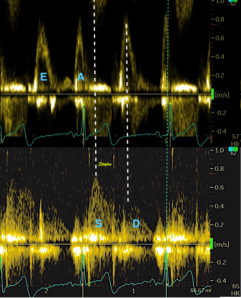
Combined mitral and pulmonary flow, showing simultaneous inflow to the LA and LV during early filling, indicating the the atrium is a conduit for the replenishment of volume to the LV.
Pulmonary venous flow visualised with CFM, showing atrial inflow during ejection (left) and early filling (middle) and a weak signal of atrial reverse flow during atrial systole (right).
This finding is the basis for the now outdated, simplified concept of the atrium as a passive conduit during this phase.
Firstly, There is longitudinal ventricular expansion and atrial compression during the early filling phase, showing a shrinking atrium, not a passive conduit:

Right: combined mitral and PV inflow, showing the concomitant venous (D) band atrioventricular flow (E) during early filling. Left, the same flows shown by colour M-mode, but also showing the AV-plane motion, with the basal motion during early filling indicating ventricular expansion and concomitant atrial compression during this phase.
Secondly, the venous inflow is dependent on transverse ventricular expansion.
The loop shows that although total outer contour is mostly unchanged, there is a systolic transverse compression as well.
The transverse expansion of the ventricles is due
to the unbending of the AV-plane and recoil of the circumferential fibre, expands
the ventricles and aspirates blood from the atria, adding to the atriovenous
flow, and is replenished from the veins.
|
|
|
During early filling there is recoil of the AV-plane, but only partly back to the end diastolic position, causing ventricularisation of part of the atrialised volume behind the compressed AV-plane (light red). This effect do not generate flow. | The unbending of the AV-plane will cause an additional reduction of the atrial volume (violet), causing pressure rise (the V-wave), and part of atrioventricular early flow. | Both undbending of the AV-plane and the recoil of circumferential fibres, will increase ventricular volume additionallly, and aspirate a further volume from atria to ventricles which has to be replenished by venous inflow to the atria (orange), the D-wave, which is the true conduit volume. |
The presence of diastolic inflow to the atria is consistent with the findings of a systolic ventricular outer volume decrease by MR, (62, 63), and by echo (7, 64, 65) due to transverse shortening, which is a function of circumferential fibre contraction, and subsequent expansion during early diastole.
As seen the systolic atrial expansion is proportional to MAPSE, meaning that the S-wave is dependent on systolic LV function (9, 175).
Nishimura et al (175) during acute reduction of preload by nitroglycerine and increase by fluid and increase of afterload by phenylephrine, that there was a strong correlation between CO and pulmonary S-wave, while both peak E and D, and the deceleration times of the two waves in the different states. Kuecherer, during cardiac surgery, found that the systolic fraction of PV flow correlated most strongly with LAP in the surgical setting (176), although the E/A ratio also did show a correlation, and likewise the changes in LAP correlated better with S fraction than E/A ratioo as well. However, both studies show mostly the effects of acute changes, and lacks data on AV-plane motion as well as atrial size.
Mitral E | Mitral A | E/A | PV S | PV D | PV S/D | |
Females | ||||||
<40 years, N=208, mean (SD) | 80 (16) | 48 (15) | 1.85 (0.76) | 58 (12) | 55 (11) | 1.09 (0.31) |
40-60 years, N=336, mean (SD) | 74 (15) | 59 (15) | 1.32 (0.40) | 59 (12) | 48 (12) | 1.29 (0.35) |
>60 years, N=119, mean (SD) | 69 (16) | 75 (18) | 0.96 (0.32) | 62 (12) | 43 (11) | 1.51 (0.39) |
All, N=663, mean (SD) | 75 (16) | 58 (18) | 1.42 (0.62) | 59 (12) | 49 (12) | 1.26 (0.37) |
Males | ||||||
<40 years, N=126, mean (SD) | 75 (15) | 44 (14) | 1.86 (0.64) | 52 (11) | 55 (12) | 0.99 (0.29) |
40-60 years, N=327, mean (SD) | 64 (15) | 52 (14) | 1.30 (0.42) | 55 (11) | 47 (11) | 1.22 (0.31) |
>60 years, N=150, mean (SD) | 61 (14) | 65 (18) | 0.99 (0.34) | 62 (13) | 43 (11) | 1.50 (0.4) |
All, N=603, mean (SD) | 66 (15) | 54 (17) | 1.34 (0.54) | 56 (12) | 48 (12) | 1.23 (0.37) |
Total | 70 (16) | 56 (18) | 1.38 (0.38) | 58 (12) | 49 (12) | 1.25 (0.37) |
As discussed under atrial strain during ejection, the atrial and ventricular strain during early filling are mirror images of each other, both dependent on the same AV plane motion as numerator.
The longitudinal compression of the atrium has been termed "conduit strain", but this is too simplistic.
Firstly, there is deformation, but the energy for that deformation is from ventricular recoil, and thus atrial deformation should have been termed: atrial strain during ventricular early filling. As for the atrial strain during early filling, it is meaningless tho consider the same AV-plane motion as a measure of atrial function viewed form the atrium, and as ventricular diastolic function viewed from the ventricle. Especially as the AV-plane velocity during early filling is the main measure of diastolic ventricular function. Again, the atrial strain during early filling is the ventricular recoil velocity as numerator, and atrial size as denominator,but atrial size may be both cause and effect related to LV diastolic function.
Secondly, as the atria compress while the ventricles expand, the pressure must decrease more in the ventricles, driving an atrioventricular gradient and flow, but the venous inflow, must be the difference between the ventricular volume expansion and atrial compression, and thus not simply flow to replenish the volume flowing into the ventricle.
Thirdly, the "atrial conduit strain" is longitudinal compression, which has not got anything to do with the replenishment volume flowing into the atria.
The early ventricular filling phase is a function of ventricular recoil. This diminishes the LA size (but is certainly not a conduit function), and the LV contribution to early transmitral flow is thus squeezing the volume from the atrium to the ventricle. The second component of early transmitral flow is the aspiration by the transverse LV expansion, and this, as additional volume flow is the conduit part, as sthis volume has to be replenished from the veins to the atria. But again the "atrial conduit function" is the function of LV early diastolic recoil. The atrial strain during early filling, is thus a composite of LV relaxation/recoil as numerator, and atrial size as denominator, so again this composite measure contains inherent confounders.
The "atrial strain curves in the "conduit phase", do not reflect the conduit volume which is the pulmonary inflow replacing part of the atrioventricular flow, but rather atrial compression during this phase. The view of the atrium as a simple conduit is much too simplistic.
Thus, the view of the early filling as a conduit phase only, is too simple.
The atrial strain during early filling, is thus a composite of LV relaxation/recoil as numerator, and atrial size as denominator, so again this composite measure contains inherent confounders.

Atrial strain curves. LASr: Left atrial reservoir strain, but the "reservoir phase" really is ventricular systole/ejection, LAScd: Left atrial conduit strain, but the "conduit phase" is in reality ventricular early filling phase, LASct: Left atrial contraction strain, the contraction phase is atrial, not ventricular contraction, i.e. atrial systole. Below are the mitral annular displacement, shown both by tissue Doppler and M-mode, seing they are nearly identical. The colour M-mode shows that the first atrial filling is the S-wave, occuring during apical annulus motion, simultaneous with the ejection, while the second filling of teh atrium actually occurs during basal AV-plane motion, i.e. atrial compression. During this phase there is atrioventricular flow due to a volume shift from atroium to ventricle, but also expansion of the ventricle, which draws more blood into the atria. But the simultaneous shrinkage of atrial volume and filling shows that this is not asimple conduit function.
Diastasis is the period between early (LV relaxation) and late (atrial contraction) filling. In fact, it is the period between the end of one heart cycle, and the start of the next (starting with the P-wave/atrialo systole/late filling).
During this phase there is little volume change and little AV-plane motion. In tissue Doppler and M-mode, the diastasis is the interval between the e' and a' waves, with no deformation. As the tissue velocities are less pressure dependent than mitral flow, the e' and a' are better separated even in delayed relaxation.
|
|
Left: normal relaxation, right, delayed relaxation. Even in delyed relaxation, there is good separation of e' and a'. Even if the early diastolic annulus velocity is reduced, so is the extent as seen by m-mode, so the e' phase is less prolonged. | Patient with delayed relaxation, showing slow, but prolonged mitral flow into diastasis, but the extent of the LV volume increase, and hence ventricular filling is reduced, due to low flow rate. Tissue Doppler still shows separation between e' and a'. |
Diastasis thus is after the recoil is finished, before atrial contraction, and show little volume change and AV-plane motion.
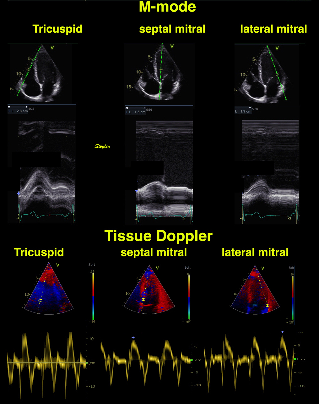
M-mode and tissue Doppler recordings, showing the diastasis between the e' and a' waves, with little or mo AV-plane motion or velocity.
In diastasis, between early filling and atrial systole, there is little AV-plane motion.
Pressure equalisasation and hence, atrioventricular flow, depends on the rate of ventricular recoil/relaxation
Relation of atrioventricular diastolic gradient and flow, showing persistence of both gradient and flow into diastasis depending on ventricular relaxation rate.
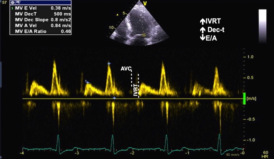
Mitral flow in delayed relaxation, showing atrioventricular flow until onset of the A wave.
In some cases, the atrioventricular pressure gradient can show a L-wave in diastasis, which signifies that the atrial pressure is elevated.
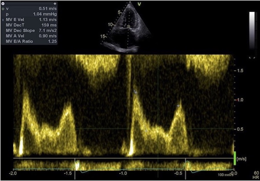
L-wave in diastasis,m signifying elevated LA pressure. The gradient is higher in early filling, due to the higher LA pressure, with a subsequent higher E-wave. But then LV pressure increases faster in response to the filling from the LA, due to both the increased filling rate, slower relaxation and finally less compliant ventricle already during diastasis. The initial dec-t is shortened, but then the flow is slowed due to decreased LV compliance, maintaining a high flow rate during diastasis.
In hemodynamic thinking, it is customary to start the heart cycle with ejection, and the to proceed to diastolic filling, hence S - E - A. This is the way tissue Doppler is presented as well. However, each heart cycle start with a sinus node activation, followed by an atrial activation and atrial systole, and this is the customary way of describing the ECG, hence P - QRS - T. But this corresponds to the sequence of A - S - E.
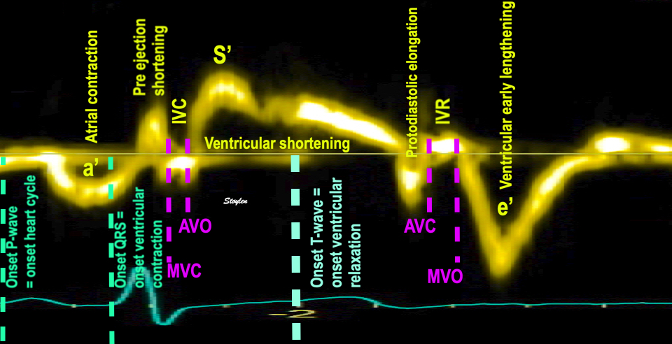
The true relation of ECG and TDI, showing how the heart cycle starts with a P and an A wave.
This may be a help in describing the relation of E and A in relation to heart rate as illustrated below.
Diastasis is in reality the interval between two heartbeats, the next heart cycle starts wit the P-wave (atrial systole).
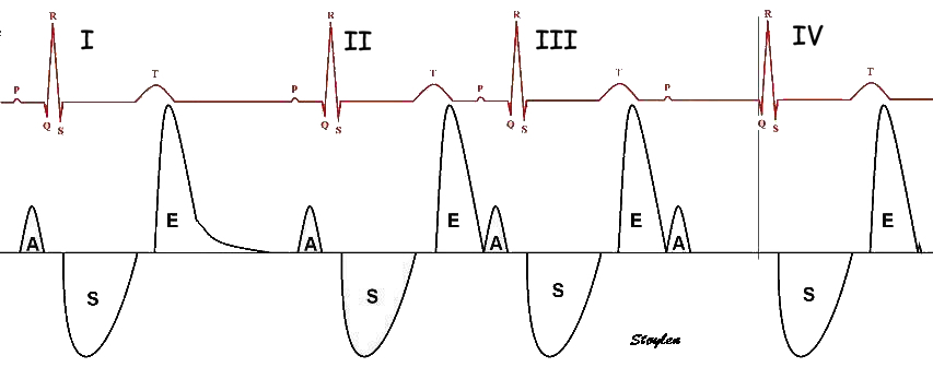
Four heart cycles illustration the relation between E and A with heart rate and PQ time. Cycle I to II show normal PQ time and RR-interval from I to II, i.e. normal heart rate, resulting in a normal diastasis period between E of I and and A of II. Cycle II to III shows shorter RR-interval, i.e. higher heart rate. As heart rate is increased, it means that P and hence A of cycle III , comes earlier after cycle II. Thus, this explains why it is the diastasis that is shortened with increasing heart rate. Cycle III to IV, shows the same RR-interval as I to II, i.e. same heart rate, but with longer PQ time. Heart rate regulation modulates the RR (or, actually PP) interval, but in this case the PQ interval is prolonged in relation to the RR interval. This has the same effect as reduced RR interval; the PQ as fraction of RR decreases, and the diastasis is abolished.
Thus, the diastasis duration depends mainly on the HR (RR-interval) and the PQ time.
however, after the diastasis interval is zero, the next step is fusion of the E and A waves as shown below:
E/A fusion with increasing heart rate (or PQ time). (NB: the numbers on this image are not related to the numbers on the image above.) 1: No fusion and discernible diastasis. 2: Shortening of RR-interval first abolishes the diastasis. 3: Further shortening of the RR-interval leads to partial fusion of the E and A wave and e' and a', respectively. the peak E and e' is still separate, but the A and a' are atrial velocities added to the remaining velocities of the early phase, as shown by the arrows in the upper diagram. In the velocity curves, this is seen as the A/a' wave "climbs" up (down) the descending limb of the E wave. 4: At higher heart rate, the E and A are completely fused, and the separate effect of ventricular relaxation ant atrial contraction can no longer be discerned.
| |
Patient with Wenckebach block, showing progressive E and A fusion as the P-wave comes closer to previous T-wave, until one beat is dropped. Prolongation of PQ-interval reduces the Q-P interval. Thus, the diastasis varies inversely with PQ-time, and the degree of EA fusion as well. | E and A with increasing heart rate during an exercise test in one patient. At HR 65,there is separate E, a and diastasis, both in mitral flow and in tissue Doppler as evident by the fact that tissue velocity is 0 between e' and a'. At HR 88 there is partial fusion, neither E nor e' reaches 0 before the start of A and a', respectively, and the A and a' are higher in absolute values due to this. At HR 94 there is more fusion, but the peak of the E and e' are still discernible, and can be measured, as a measure of ventricular diastolic function. The E/A and e'/a' ratios, however, are useless, as the A and a' are summation velocities. The A and a' are increased further. At HR 121, the E/A and e'/a', respectively, are nearly completely fused. The peak E and e' can no longer be discerned. The peak diastolic velocity is far higher (in absolute values) that the E or e' and cannot be compared. |
In a study of time intervals during exercise (225), the findings had relevance for the phenomenon of the E/A fusion. As heart rate increases, it is the diastasis that is shortened first as this is the interval between heartbeats. Thus, the RR-interval and the diastolic filling period (E, A and diastiasis) shortens in parallel, while the ejection period shortens more slowly (225). This is the function of the shortening of the PQ interval, until there is EA fusion. After EA fusion, DFP and LVET shortens in parallel, both semingly linearly, but the decrease in RR-interval
|
|
Left ventricular diastolic filling period (DFP) and ejection period (LVET) in relation to heart rate during exercise. Below HR 110, the RR interval and DFP shortens in parallel, showing the the diastasis is shortened first, while ejection time shortens much less. Above 110, there is parallel shortening of LVET and DFP, both contributing to the shortening of RR interval. | Comparing the intervals with the RR interval, makes the relation more evident: The DFP decreases more or less linearly, more rapidly than LVET down to about RR interval of 580, from there both LVET and DFP decreases in parallel, and LVET more raapidly than above 580. |
All intervals of the heart cycle shortens relative to increasing heart rate, but below 100, RR-interval and DFP shortens mainly by reduction of diastasis. Above 110, diastasis is zero, with fusion of the E and A waves, and hence all intervals shorten in parallel. Thus, the ejection period curve has a nonlinear relation with RR-interval, with a break at RR interval of 580. The linear correction for LVET by HR proposed by Weissler (226), thus is only valid up to HR about 100. Interestingly, the older, nonlinear square root HR correction proposed by Bazett (227), as the Weissler formula, by linear regression showed an increase in the corrected LVET, Basett's formula gave similar corrected values across the whole range of HR values (225). This doesn't necessary mean that the square root correction is true, but it takes the non lineariyt of LVET into account, with the break around 100 (but there may be linearity both below and above).
After early filling, the vortex has filled the whole ventricle. The vortex persists into the diastasis, and closure of the anterior mitral leaflet by the septal, basally directed part, may even conserve the vortex energy during this phase, allowing vortex flow to pass from the downward part to the upward part aligning with the atrial systolic inflow.. The flow along the lateral wall is apically directed, and will conserve momentum from the base, into the late filling period, again adding kinetic energy to the kinetic energy from atrial systole during this phase.
| |||
Septal M-mode showing basally directed flow, during diastasis contributing to partial closure of mitral valve. | Image during early diastasis, showing persistence of the vortex generated during early filling, and beginning partial closure of the anterior mitral leaflet.Image courtesy of Annichen S Daae. | Image during late diastasis, showing persistence of the vortex, and alignment of the lateral part of the vortex and the beginning of inflow during atrial systole.Image courtesy of Annichen S Daae. | Lateral M-mode showing apically directed flow during diastasis, before atrial systole, but aligning with the inflow in late filling. |
In this phase, vorticity between the E and A waves remains higher, but decreases during diastasis, reaching a nadir before the A-wave.
During diastasis, vorticity remains higher, despite a drop in kinetic energy, which may be a mechanism for transfer of momentum to the A-wave.
The late filling is the atrial contraction.
As each heart cycle start with a sinus node activation followed by an atrial activation , hence P - QRS - T, and then atrial systole, this corresponds to the sequence of A - S - E.
Thus, the atrial contraction is the first part of the heart cycle.
The true relation of ECG and TDI, showing how the heart cycle starts with a P and an A wave.
The AV-plane is pulled basally from the diastasis position after end of the recoil.
It has been suggested that the main function of the atrial contraction is the lifting of the AV-plane toward the base. However, if this had been the main mechanism, it would result in pressure drop in the ventricle, while the reality is that pressure rises both in atria and ventricles during atrial systole, showing clearly that the mechanism for the AV-plane motion is longitudinal ventricular expansion due to the volume injected into the ventricle.
In addition, the atrial contraction also includes the emptying of the atrial appendages. This is not part of the direct atrial muscle effect on the AV-plane, but of course, the volume effect of atrial emptying into the the ventricles will move the AV-plane, so the appendaghes' contraction is still, though indirectly reflected in AV-plane motion.
|
|
During atrial contraction (the start of the heart cycle), The AV-plane reverts to the end diastolic position. This basal motion | Diagram of the heart, showing the atrial appendages, and the flow of blood into the atrial cavities. Contraction of the appendices, part of the atrial volume reduction during atrial systole, contributing to the volume injected into the ventricles.Thus the atrial appendices inject blood into the atria, and with open atrioventricular valves also into the ventricles, hence, the AV-plane motion also reflects the appendices' contraction. |
|
| |
Pressure curves showing atrial and ventricular pressure rise during atrial systole, indicating that the ventricular volume expansion is due to the volume injection into the ventricle by the atrial contraction.During atrial systole, there is pressure increase in both atrial and ventricles. The AV-plane motion (and atrial contraction strain) is an incomplete view of the atrial deformation, however, that do not take the atrial appendages into consideration. During atrial contraction, the appendiceses contract too, injecting their volume into the atrial cavity, causing pressure rise, both in the atria and ventricles, and atrio venjtricular volume flow. This volume is what expands the ventricles and moves the AV plane. But the simultaneous increase in atrial pressure, would also cause a reverse flow from the atria to the veins (the A flow wave). | Atrial /red), left ventricular (blue), Pulmonary venous (magenta) and pulmonary artery (green) pressure curves. a: atrial pressure rise during atrial contraction. z: pressure decline after a. c: Initial atrial pressure rise at start systole x: pressure decline during LV ejection V: pressure rise at end ejection. |
The pressure curves indicate a pressure rise in both atria and ventricles during atrial systole. The ventricular pressure rise is the end diastolic pressure volume relation, a function of ventricular compliance.
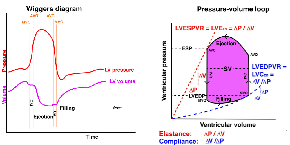
Looking at the ventricular end diastole, we see there is pressure rise due to atrial contraction, and the pressure rise is a function of the atrial emptying volume, and the ventricular compliance.
In this phase, it seems that atrial contraction actually leads to ventricular stretch, thus it is not related to recoil from ventricular systole, as shown by the lack of correlation between MAPSE and a' and S' and a' in the HUNT3 study (156). Thus, the ventricular end diastolic elastance, is impedance to ventricular filling.
However, the atria have double outlets during atrial systole, with both atrioventricular orifices and veins open at the same time. Veins being without valves, and being compliant, would offer far less impedance to the atrial pumping, and would have absorbed most of the volume output of the atria, if there had not been some sort of impedance matching between veins and ventricles.
However, it has been demonstrated that the atrial musculature extends into the venous walls in the form of myocardial sleeves, at least 15 mm out into the veins from the ostia (255, 256). The venous myocardium, being contiguous with the atrium, will contract during atrial systole. This contraction has been demonstrated by MR (257) and by CT (258, 259), with minimum venous area during atrial systole.
It has been suggested that this will increase the resistance to venous backflow during atrial systole. However, pulmonary veins, being rather large, are not resistance vessels. More probable, the volume reduction, as well as the wall stiffening, will both increase venous compliance during atrial systole, thus increase the pressure during the venous venous backflow that demonstrably is present (61). Pressure increase during atrial systole is demonstrated (157), consistently with this (resistive impedance would limit flow, by limiting the atrial venous difference, capacitative impedance limits flow by pressure increase).
The amount of volume injected intot he ventricle, is firstly dependent on the amount of filling during early diastole, i.e. LV relaxation. Reduced relaxation gives reduced early filling (E), and hence increased late filling, increasing the A of the EA ratio:
|
|
|
|
Relation between mitral flow indices and pressure in the normal situation. Early mitral flow (red curve) is dependent on the pressure gradients between the left ventricle and the atrium, which is created by left ventricular relaxation. Atrial pressure increases during atrial systole, forcing blood to flow again in the A wave. | Slower relaxation leads to a less profound but longer drop in LV pressure, leading to a reduced E amplitude . The lower filling volume leads to a higher atrial volume at the start of atrial contraction, and thus a higher atrial stroke volume (perhaps by the Frank-Starling mechanism), and a higher A- wave. The E/A ratio is reversed. (Light gray flow curve is from A, for comparison). |
However, the ventricular filling during atrial systole, also depends on the end diastolic compliance. Compliance is the amount of volume expansion per pressure increase: C = ![]() V /
V / ![]() P. The lower the compliance, the less volume is injected into the ventricle.
P. The lower the compliance, the less volume is injected into the ventricle.
|
|
|
LV end diastolic compliance, shown in a pressure volume diagram. As we see, early diastole is the active relaxation (recoil), generating ventricular pressure drop and volume expansion, thus the compliance is negative. In end diastole there is atrial contraction grenerating pressure increase and volume expansion, thus positive compliance. | Decreased LV compliance, meaning that for the same pressure increase, there is less volume expansion (or for the same volume expansion, there must be generated more pressure), shown by the less filling and steeper pressure volume curve. | With decreased LV compliance, the pressure increases more, during atrial systole, and despite this, fills the ventricle with less volume. |
However, the atrial have double outlets, both into the ventricles as well as into the veins. During atrial contraction, blood flows both forwards into the ventricles, and backwards into the veins. However, it has been demonstrated that the atrial conrtraction narrows the venous orifices (229), thus increasing the venous impedance as the ventricular pressure increases. Thus the retrograde flow tends to be reduced by impedance matching.
Pulmonary venous flow visualised with CFM, showing atrial inflow during ejection (left) and early filling (middle) and a weak signal of atrial reverse flow during atrial systole (right).
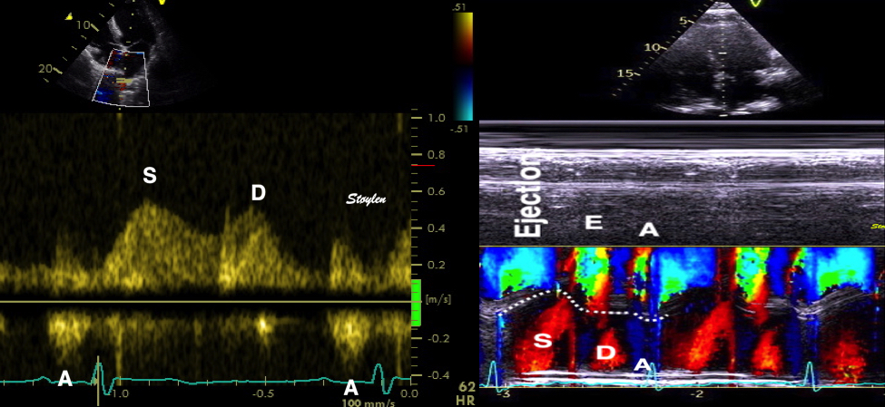
Pulmonary venous flow, showing the normal reverse flow into the veins during atrial systole.
The veins are low pressures. The atrial pressures are nearly equal to the venous pressures, but the atrial pressure increase generated by the atrial systole, will drive the flow both forwards and backwards. The flow into the ventricle is then decelerated by the intraventricular pressure increase, and the pressure increase per volume increase is a function of ventricular compliance. Thus, if the inflow into the ventricle stops earlier due to reduced compliance, while the venous backflow continues due to the lower pressure, there is a discrepancy at the end of the two a-waves. A 340 ms longer duration of the pulmonary A-wave than of the mitral A-wave is considered a criterion of elevated LV end diastolic pressure (61).
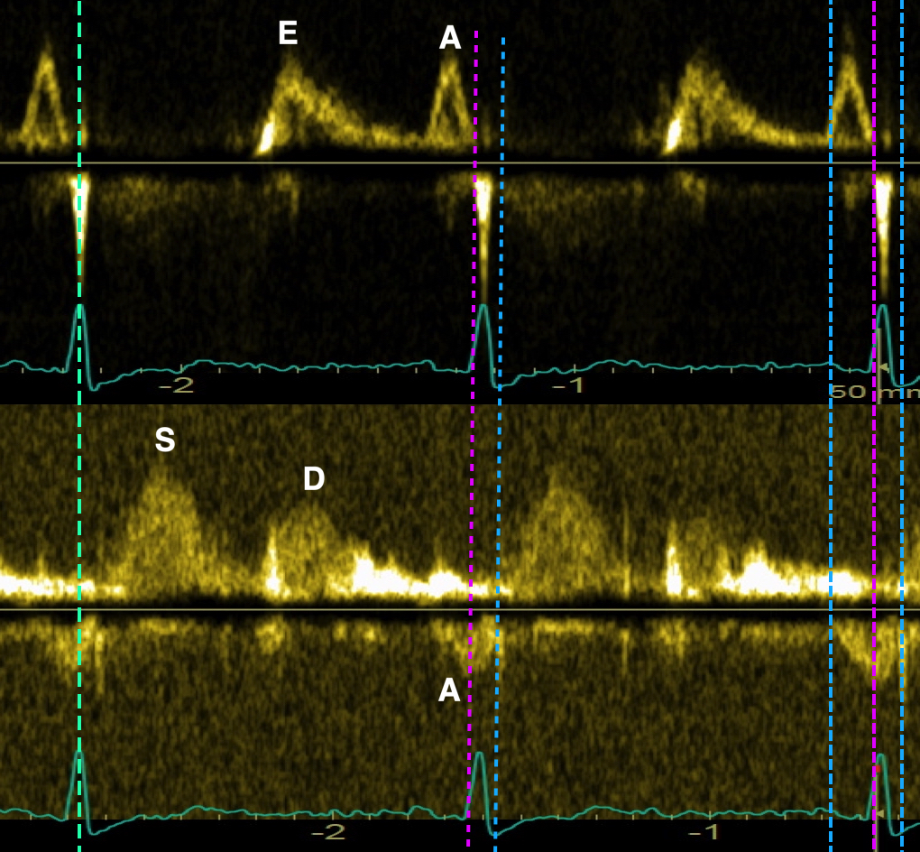
Mitral and pulmonary venous flow from the same patient, aligned by ECG (cyan bar, left). By the ECG, the A wave of mitral flow can be seen to end before the peak R, while the A wave of PV flow ends after the R-wave. the end points are indicated in the middle heartbeat, the A of mitral flow shown by the magenta bar, the PV A wave by the blue bar. Finally, for comprehensive analysis, the full duration of the A waves are shown in the last heartbeat, mitral A lasting from the blue to the magenta bar, PV A wave between the two blue bars. A PV A duration of > 30 ms more than the mitral A is considered significant. However, the end points are the main difference.
As the AV-plane motion during atrial systole, reflects the ventricular expansion, which is due to the volume effect of atrial contraction (including the contraction of the appendices). Thus, the AV plane motion reflects the total atrial contraction function, including the appendages.
The late filling phase is also the atrial contraction phase. Atrial contraction, is thus one determinant of the AV-plane motion, and atrial contractility will increase the AV-plane motion (atrial strain ).
However, the AV-plane motion, being a measure of ventricular volume expansion, is also dependent on the ventricular compliance. Compliance is the amount of volume expansion per pressure increase: C = ![]() V /
V / ![]() P. The lower the compliance, the less volume expansion, AV-plane motion/lower Atrial contraction strain.
P. The lower the compliance, the less volume expansion, AV-plane motion/lower Atrial contraction strain.
Thus, the atrial contraction strain is a function of atrial contraction, but also of LV end diastolic compliance, and always with the atrial size as denominator. LV expansion is more uncertain, as the atria have double outlets.
The late filling phase is also the atrial contraction phase. Atrial contraction, is thus one determinant of the AV-plane motion, and atrial contractility will increase the AV-plane motion (atrial strain ).
However, the AV-plane motion, being a measure of ventricular volume expansion, is also dependent on the ventricular compliance. Compliance is the amount of volume expansion per pressure increase: C = ![]() V /
V / ![]() P. The lower the compliance, the less volume expansion, AV-plane motion/lower Atrial contraction strain.
P. The lower the compliance, the less volume expansion, AV-plane motion/lower Atrial contraction strain.
Thus, the atrial contraction strain is a function of atrial contraction, but also of LV end diastolic compliance as numerators, and always with the atrial size as denominator.
During late filling the vortex cycle from early filling repeats somewhat, there is:
Downwards movement of the AV-plane.
Diversion of the inflow into LVOT by the same mechanism. The basal motion of the AV-plane again will expand the LVOT, diverting blood towards the septum and downwards, creating a new vortex similarly to the early filling, which also originates near the ventricular base.This is visible both by colour and pwDoppler:
|
|
|
Inflow into LVOT relates to the AV-plane motion, both during early and late diastole | Late diastolic vortex forms close to the base by deflection of inflow into LVOT, related to the AV-plane motion. Image courtesy of Annichen S Daae. | Inflow is thus mainly in the lateral part of the ventricle. |
This again creates into the LVOT, immediately before ejection. Earlier described as the “J-wave”(488), though incorrectly taken as return of the E-wave via apex. However, the paper correctly, but
inconsistently related the peak of the J-wave as related to the mitral A-wave and EA ratio.:
LVOT inflow pattern in a patient with a low E/A ratio, and it it evident that the LVOT E/A ratio, and thus the height of the J-wave reflects the mitral E/A.
The transit time of the A wave into the LVOT has been found to be shorter than the transit time of the E-wave (229), 20 - 80 ms as compared to 80 - 200 ms.
In a recent publication the A_LVOT was described as “pre systolic flow”, reported in only a fraction of patents, irrespective of EF, but presence associated with worse prognosis. However, this is in discrepance with the finding that the pre systolic flow is normal physiology. As the amplitude of the A_LVOT is associated with the E/A ratio, low detection of A_LVOT may be related to the amplitude, creating a bias in detection towards a high E/A ratio, and thus being a confounder.
Late inflow runs into a pre existing vortex, while early inflow runs into an apically directed momentum. While the septal part of the early vortex seems to weaken, inflow in the A wave
aligns with the lateral part, as the same time as the new vortex expands towards the apex.
|
|
|
Successive imagesof vortex flow in last part of diastole. The vortex is present before late filling, but increases during the filling, so vorticity is visibly increased after late filling. Images courtesy of Annichen S Daae. | ||
diastasis at the point of mitral valve re opening | full inflow during late filling | end of filling /pre ejection after MV closure. |
Vorticity, of course increases with the formation of this new vortex, again slightly belated after the peak A-wave (kinetic energy).
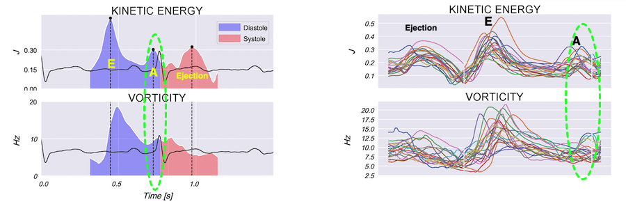
Increase in vorticity just after the peak kinetic energy of the A-wave.
And then the cycle repeats at pre ejection:
|
|
|
Septal colour M-mode showing basally directed flow along the septum during PEP. It can be seen to start at the beginning of MV closure. | Vector flow imaging, showing the intraventricular counterclockwise vortex during pre ejection. The finding is consistent with the colour M-mode findings. Image courtesy of Annichen S Daae. | Lateral colour M-mode showing apically directed flow along the lateral wall during PEP. |
The Wiggers diagram is an illustration of temporal relations of atrial, ventricular and aortic pressures with ventricular volumes, in a simplified, schematic illustration of the main relations, for basic teaching purposes. However, as the previous chapters have shown this a very simplified version, and thus not the full truth. It does not at all regard the the effects of inertia of blood, nor the knowledge from newer physiological studies with high-fidelity catheters, nor from Doppler and TDI. This will affect the form of the diagram:
Pre ejection shows a small shortening before MVC as explained here. Protodiastole shows a small lengthening before AVC as explained here. Thus the isovolumic phases are shorter than depicted, and the volume curve not as smooth.
Blood does not always flow from higher to lower pressure, the inertia of blood means that stationary blood will be accelerated by a positive gradient (along the flow direction), and flowing blood decelerated by a negative gradient (opposite to the blood flow), and this means that both atrial systole, ejection and early filling, showing acceleration of flow velocity from zero to peak, and the deceleration from peak to zero, will have biphasic pressure gradients.
In addition, the inertia of the blood means that the LV volume curve is sigmoid, not through shaped as traditionally depicted.
|
|
The traditional form of the Wiggers diagram. The weaknesstes of this, is that it depicts blood as only flowing from higher to lower pressure, and peak volume decrease during e3jection to be steepest at AVO. | Wiggers diagram with added flow velocity curves, and adjusted for:
|
Segmental strain do not only reflect segmental contractility, but also interaction with other segments.
Both differences in onset of tension, different tension during contraction and differences in timing will give segmental inequalities in shortening.Simultaneous shortening of one part of the ventricle and and stretching of another, occurs when there is tension imbalance.
This may occur physiologically during the IVR (72), and in regional dysfunction, mainly in regional ischemia as discussed below, and in conduction disturbances
Regional strain is also about regional differences in local load:
|
|
|
Length tension diagram of a muscle twitch in an isolated muscle preparation. The muscle takes some time to develop the tension that equals the load, and during that period the contraction is isometric, with no shortening. Shortening starts when tension equals load. When the muscle relaxes, relaxation induces shortening until tension again equals load, after that relaxation is isometric. | Series of twitches with different loads. All twitches follow the same tension curve, i.e. shows the same contractility, but as load increases, shortening starts at later time points, and the shortening time as well as the extent and rate of shortening decrease. | Series of twitches with the same load, but with different contractility (ability to develop tension). With decreasing contractility, it takes longer to develop tension = load, the period of shortening as well as the extent and rate of shortening decrease. |
Regional differences in strain rate and strain arises from two mechanisms:
|
|
Illustration of how all segments in a normal ventricle (here illustrated in a two-level model) can generate the same tension, and the same segmental shortening, but the added shortening from the apical segments will generate more motion of the the basal segments by tethering, and thus explains the motion and velocity gradient from base to apex. | Top: segmental shortening of the septum, left :strain rate, right: strain. Bottom, the resulting motion of the segmental borders, where the apical shortening pulls the midwall and basal segments along, imparting motion, and the midwall segmental shortening imparts an additional motion to the basal segments. Left velocities, right displacement. |
Each normal segment develops nearly equal tension, and thus confers equal load to the other segments, so shortening is also equal in all segments (although displacements are not).
As discussed in the section on global strain, wall thickening (transmural strain) is mainly a function of wall shortening (7). This must, for geometrical reasons also be the case for segmental strain, and we have also shown this to be the case in clinical diagnosis (195 - 197). Thus, wall thickening and wall shortening are equivalent. The regional systolic function is traditionally shown as wall motion score:
This was originally given from wall thickening, but we showed that it could just as well be applied to the semi-quantitative colour strain rate display (196), and that they were equivalent regarding information (197)
|
| I |
Segmental division of the left ventricle. The segments are related to different vascular territories, as shown by the colours. However, in the figure given in that paper, the apicolateral segment is given as Cx or LAD, while the apical inferolateral is not, despite the model is only giving four segments in the apex. Thus, there is a slight inconsistency. | n WMS = 2, there is both hypokinesia and tardokinesia as well as PSS, in WMS 3 there is PSS and in WMS=4, there is dyskinesia and PSS in the apical segment, but also PSS inthe midwall segment indicating a more extensive partial ischemia. |
Wall motion score index (WMSI), being the average of wall motion score of all evaluable segments becomes a measure of global function, and has been shown to correlate with EF in infarcted ventricles (126). However, the index is useless unless there is regional differences. Any dilated cardiomyopathy will show hypokinesia in all segments, giving a WMSI of 2, regardless of EF. Thus, wall motion score is useful only in regional dysfunction.
Segmental dysfunction results in reduced segmental tension. This is usually due to ischemic heart disease, and may result from
The tension of each segment, is part of the afterload of the neighboring segments, which, if normal, will increase shortening, while the weakened segment will reduce shortening. In addition diastolic regional finction will change, because relaxation is energy demanding, so relaxation will last longer in an ischemic segment, and thus the seg,ment will remain under tension when the normal segment has finished shortening, so the tension in the ischemic segment, having been offloaded, will shorten - post systolic shortening PSS.
This can also be recognised by the separation of the velocity or displacement curves.
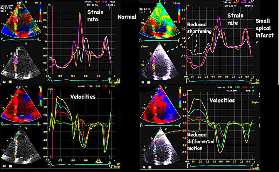
Left: Normal ventricle, right: small apical infarct, top: strain rate, below: velocity curves. In the normal ventricle, the systolic strain rate can be seen to be relatively similar in all three segments, about - 0.9 s-1. This corresponds to a relatively even spacing of the velocity curves. In the infarcted ventricle the apical segment can be seen to have strain rate of about - 0.5 s-1, compared to the normal strain rate of -1s-1 in the midwall and basal segments. Looking at the velocity curves below, the two points bordering the apical segment (red and green) can be seen to be very close to each other, indicating that they move as a stiff piece without deformation.
Just inspecting the velocity curves is thus a way of visualising the strain rate without measuring it.
Regional load is not only systolic pressure, but also the tension in the neighboring segment, so if the contractility of one segment is reduced, another segment experiences less load, and thus will shorten more
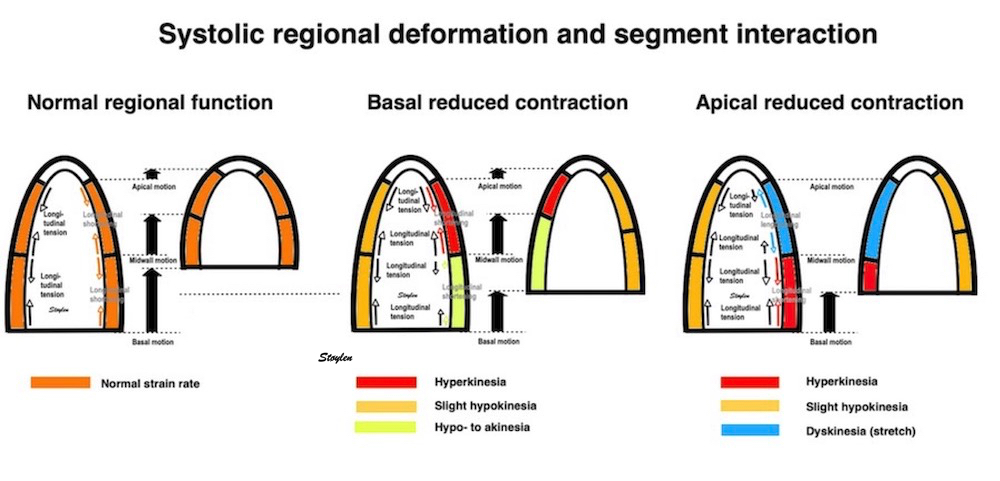
Diagram over segmental interaksjon ved redusert regional kontraktilitet. dette gir redusert tensjon (og derved load), på nabosegmentet, som derved vil forkorte seg mer, TOTAL forkortning, derimot, vil gå ned som følge av redusert toital tensjon, som indikert med de svarte pilene.
The interaction between segments was demonstrated in post infarct recovery studies (182, 183). If there is initial hypo- to akinesia in infarcted segments, there is corresponding hyperkinesia in neighbouring non infarcted segments. As contractility in infarct segments improve due to recovery of the stunning part of the injury, the resiproke hyperkinesia will regress as illustrated below.
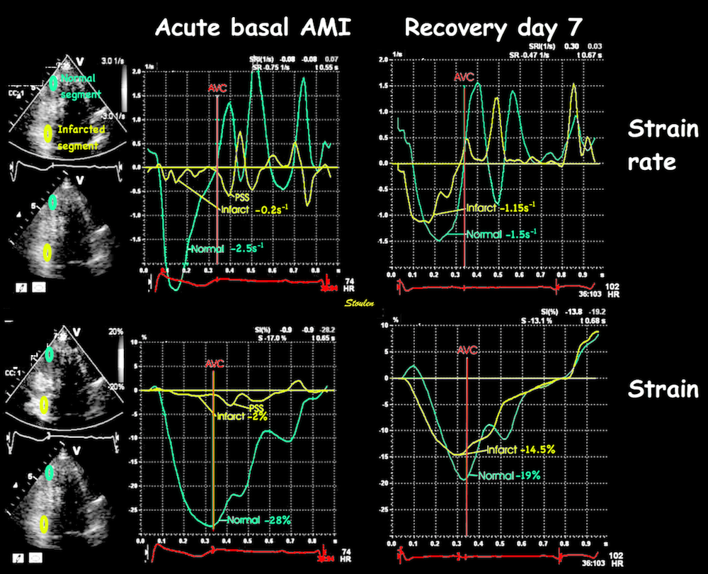
Strain rate (A, B) and strain (D, E), of an inferior infarct at day 1 (A, D) and Day 7 after successful acute PCI (B, E). There is akinesia in the basal segment (yellow curve) and hyperkinesia in the apex (cyan curve). The hyperkiesia can be explained by the load reduction due to the lack of force from the infarcted segment. The same patient At day 7 function in the basal segment (yellow curve) can be seen to be nearly normalised, and the shortening of the apical segment (blue curve) is correspondingly reduced.
Thus, differences in contractility will affect both normal and pathological segments, and in various ways depending on the amount of weakening and localisation:
|
|
|
|
|
Symmetrical forces in all segments, will result in symmetrical shortening. Thus, all segments shorten equally (orange colour), which means that the base moves most (the sum of shortening of all segments), as the apex is stationary. | Loss of contractility in a basal segment (smaller black arrows in the left basal segment), results in less shortening in the affected segment. However, this means that the load on the more apical segment is reduced, and thus, this segment will shorten more (Red colour), not due to hypercontractility, but to less load. Also, the total force acting on the base is reduced, resulting in reduced total shortening (smaller red arrows in the base). | Even more reduced tension in a basal segment will result in the segment actually stretching, while the apical segment shortens even more in response to the basal segment stretches. This will not result in reduced motion of the regional mitral ring point, mainly a shift in the distribution of shortening between segments, and a reduced global shortening. | Reduced tension and stretch of an apical segment may result in increased shortening of the opposing wall, as well as the basal segment, but this may result in a rocking of the apex toward the healthy wall. | Symmetrical weakening of the apical segments, may result in increased shortening of the basal segments, but as the apex stretches, the motion of the AV-plane is more reduced. |
below is compared a case of pseudodyskinesia due to external LV compression with a case of true dyskinesia due to an infarct.
|
|
Pseudodyskinesia due to external compression of the inferiolateral wall. The patient had a lymphoma, and was assessed before cytotoxic therapy. The finding was reportad as an infarct sequelae. Lucily, the oncologists had more sense than the cardiologists so they went on with chemotherapy anyway. | Patient with true dyskinesia. But not in then inferolateral wall as it mighe look like, but in the apex. |
|
|
No sign of dyskinesia in strain rate imaging, the wall shortens normally as seen by the colour, evemn though there is some recoil due to abnormal mechanics. | Evident apical dyskinesia, midwall hypokinesia and post systolic shortening in both, giving the impression of inferior wall dyskinesia. |
In this case, the strain rate imaging is useful to rule out the apparent dyskinesia in the left case, and to localise the pathology in the right case. The dyskinesia is in the apex on the right, causing the visual dyssynchrony between the apex and the base. The patient had an LAD infarct.
Looking closer at the pseudodyskinetic case:
|
| |
Parasternal long axis view. Inferolateral wall looks evidently dyskinetic. (However, the normal wall thickness gives a reason to be suspicious.) The finding is the same as in the apical long axis view. | Apical two-chamber view. Basal inferior wall also looks definitely dyskinetic, although in this view out-of-plane motion is very often present. | Parasternal short axis. Again, the paradoxical motion of the inferior wall is evident, but looking more closely, this is due to diastolic flattening, with an outward motion to a closer to normal normal circular cross section in systole. Thus, there is no evidence of systolic bulging as in true dyskinesia, and the pseudodyskinesia becomes evident in this view. |
|
|
|
In the apicalal strain rate image , there is no evidence of dyskinesia, which would show up as longitudinal stretch (blue). | Neither is there dyskinesia in the two chamber strain rate analysis. | Reconstructed M-mode through the inferior wall from the same loop as above. The inferior wall shows normal systolic thickening. As wall thickening and wall shortening are equivalent, the M-mode gives transmural strain, and confirm normal myocardial systolic deformation. |
In this case, it is evident that this is not dyskinesia. The paradoxical motion is due to diastolic inward motion, and was due to compression from the outside. This was due to external compression from lymph nodes in the mediastinum.
After cytostatic treatment, the pseudo-dyskinesia was gone:

Before and after 3 months of chemotherapy. The pseudodykinesia is gone, as the tumpour is reduced in size.
A corollary of the fact that segmental shortening balance through load, is that the ring motion is not affected regionally, only globally. This was first shown by us in 2003 (126).
In a study of 19 infarct patients versus 19 control subjects, we found that while global function was reduced in patients, the variability between the difference between annular points was not:
As strain and strain rate are noisy methods, it is an attractive thought thay annular measures (annular systolic displacement or velocity) will give some regional information, in that points on the mitral ring close to a hypo- or akinetic area will show reduced motion, while remote points will not, but this is definitely not the case.
In a study of 19 infarct patients versus 19 control subjects, we found that while global function was reduced in patients, the variability between the difference between annular points was not:
Mean | ||||||
EF (%) | WMSI | MAE(mm) | S' (cm/s pwTDI) | S' (cm/s cTDI) | Segmental SRs (s-1) | |
Patients: | 41 | 1.6 | 1.2 | 7.7 | 4.8 | 1.0 |
Controls: | 55* | 1* | 1.6* | 9.9* | 7.6* | 1.4* |
Mean intra subject variation (max - min) | ||||||
Patients: | 0.41 | 2.8 | 2.5 | 1.6 | ||
Controls: | 0.41 | 3.4 | 2.8 | 1.0* | ||
Thus, no ring measures showed increased variability in infarct patients who had regional dysfunction. Only the segmental measure of strain rate did show that, despite having the highest variability. Moreover, in the patients; there were no differences between the magnitude of ring measures close to the infarct, compared to the measures remote from the infarct:
MAE(mm) | S' (cm/s pwTDI) | S' (cm/s cTDI) | Segmental SRs (s-1) | Mean SRs (s-1) per wall | |
Close: | 1.2 | 7.7 | 4.9 | 0.8 | 1.0 |
Remote: | 1.2 | 7.2 | 5.1 | 1.1* | 1.1 |
The mitral ring motion were reduced in infarct patients compared to controls, and more reduced in anterior than in inferior infarcts due to the difference in infarct size.Thus, it can not be inferred that the point on the ring close to the infarct can identify the affected wall.Only the segmental measure did show difference between close and remote points, while the ring measures did not. And finally, averaging all three segments in a wall, resulting in a wall measure equivalent to the ring measures, made this difference disappear. This means that ring measures all are global measures, local reduction of contractility will affect segmental shortening, but not local ring motion. This has been confirmed in an MR study (184).
The global systolic motion of the ring is a measure of the infarct size (185), being reduced in proportion to the total amount of longitudinal fibre loss (186). Segmental reduced function will not cause the ring to lag in part of the circumference, however, the total ring motion will be reduced as a function of the reduced total shortening force. This may explain why the global strain is just as useful as regional strain in assessing the total infarct size (187).
Another patient shows the same segmental interaction, and with no effect on the regional mitral ring motion:
Day 1:
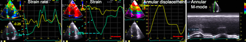
Patient with a small apical infarct at admission, showing reduced strain rate of - 0.25s-1, and strain of -2% in the apical segment (yellow), with slightly high strain ate and strain (-1.3s-1 and -25%, repectively) in the basal segments (cyan). Mitral ring motion is 16 mm, both by tissue tracking (integrated velocity, and by annular M-mode.
Day 7:
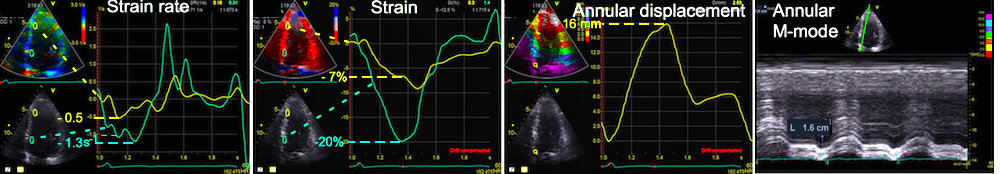
Same patient after sucessful PCI of the LAD. There is moderate recovery of contractility in the apical segment (to peak strain rate - 0.5s-1 and peak strain - 7%). There is decrease in basal strain to 20%. Peak strain rate do not seem to have decreased, but as strain rate is instantaneous, we see that strain rate in the base at the time of peak strain rate in the apex has decreased to - 1s-1. The reciprocal changes in strain in the two segments results in no change in the regional annulus motion which still is 16 mm by both methods.
As we have seen above, the PV loop represent the global myocardial work, where myocardial tension is mostly related to pressure, while myocardial shortening is related to volume.
Going back to isolated muscle preparations, it was shown early that the tension-length loop was very similar to the pressure volume loop, seen in intact hearts, and also correlated very closely with oxygen consumption (188). Measuring segmental myocardial length in open heart animal experiments, it was also shown that as the shortening decreased in myocardial ischemia, the segmental end systolic pressure-length relation and the length-pressure loop decreased (189), and also that the segment length loop correlated with estimated segmental work (190).
As segment length changes are equivalent with strain, the segmental strain-stress loop, even without strain imaging thus cold be shown to be equivalent with segmental myocrdial oxygen consumption in an elaborate experimental setup (191) in whole ventricles as well, and myocardial blood flow and oxygen consumption was much lower in early than late activated segments during asynchronous pacing..
Glower (192) showed that there was a very close parallel between the findings from pressure volume loops and pressure strain loops from segmental strain. Thus again, demonstrating a close relation between strain and stroke volume. This means, that the pressure-strain loops in a symmetric ventricle, may be a measure of regional myocardial work (193).
With strain imaging, regional strain pressure loops can be estimated (194).
It does not take diastole into consideration, as the normalised curve is based on normal diastolic pressures, so neither relaxation or compliance differences will be taken into account. Neither will pressure augmentation.
Various method for estimating DBP have been tried as well, based on models, or on databases. However, model estimates are only valid for the population where they are validated, and especially estimating of diastolic pressure is not valid in ischemia without having been validated in ischemic models or populations, as diastology changes in ischemia, especially by PSS.
E/e' has been applied as a correction for elevated DBP. ref. However, while this is a marker for elevated LAP, and thus LV mid diastolic pressure, it is not a linear relation.
As argued by the authors, systematic errors in pressure estimation does not matter when regions are compared, as the error will be the same for all regions. However, a corollary of this is that the differences in regional pressure - strain loops between segments are solely described by the differences in strain, as the pressure curve is the same for all segments. Thus, segmental myocardial work does not add information. Thios is shown in the diagram below.

Construction of regional strain pressure loops. A standardised pressure curve, is calibrated in time by valve opening and closures, and in height by arm cuff BP. With regional strain curves, regional strain-pressure loops can be constructed, and the illustrations to the left shows how the loop is different in a normal segment and an ischemic segment. But the height of the PV loop is equal to the pressure, and the width is equal to the regional systolic strain. And as the different segment loops are derived from the same pressure curve, they have the same height, the only difference in the loops are actually the strain, and the different width of the loops equals the peak systolic strain.
As the difference between segments are only the strain, while the pressure curve is the same, only the strain carries the information of the difference in regional function. Thus, this is actually the Emperor's new clothes. And the method will be just as sensitive to noise, as regional strain, of course. However, as discussed above, in regional dyssynergy, there is work done by segments when they shorten, by stretching other segments during part of the heart cycle, without concomitant change in pressure. This is the result of the segment interaction being part of the segmental load. But this means that there is an assymmetric relation between segments.
As a segment becomes ischemic, there will be reduced energy (ATP) available, this will lead to:
But the deformation pattern of the ischemic segment is then a result of this process in interaction with non-ischemic segments. Below is a sequence of diagrams of segment interaction where slower tension buildup, lower total tension and slower tension devolution is illustrated in terms of interaction with normal segments.
|
|
|
|
|
Two segments with equal tension (red and blue) will shorten equally and symmetrically. | If one segment (blue) becomes ischemic, this will lead to: | As ischemia progresses and tension becomes lower, the initial stretch increases,and shortening becomes less and later, while post systolic shortening remains. | At one point, there will be only stretch during systole. However, the remaining post systolic shortening after normal contraction, is a sign that there is still active tension remaining. | Finally, with total loss of tension, there is only stretch. The post systolic shortening is still present, but only as a recoil phenomenon, with no sign of active tension in the ischemic segment. |
|
|
|
|
Example from a real stress echo, as described in full below. The cyan curve is apicolateral segment, which is maximally ischemic, and shows conformance to the model above. The red curve is basal septal, which conforms bst to the non/ischemic segment, while the yellow curve is apicoseptal, and ischemic, although to a lesser degree. The white vertical line shows the AVC.
The full deformation pattern in acute ischemia was shown early in the experimental work of Tennant and Wiggers (177):
|
|
Time course of segmental myocardial deformation after acute LAD occlusion. The deformation (myogram) curves have been inverted to orient them as customary for strain curves today. Thus, the sequence starts at the bottom with A, and progression of ischemia is upwards, following the letters to the left. The numbers to the right, denotes the number of heartbeats after occlusion. As we see, in A there is a normal strain curve, the first change is an abbreviation (B) of the duration, and then delayed onset and reduction of the magnitude systolic strain (D), followed by initial systolic stretch and an increasing post systolic shortening peak (E-G). At the end, the systolic stretch lasts through systole - i.e. holosystolic stretch, but with post systolic shortening that exceeds the amount of systolic stretch )H-J), and finally there is virtually only passive stretch and recoil (K). | Myocardial ischemia in the LAD area during dobutamine stress echo shown by the strain curves. The different colours of the curves correspond to differently placed ROIs in the lateral apex (cyan), septal apex (yellow) and basal septum (red). To correspond to the image to the left, the time course of ischemia is from bottom to top, so the four panels are baseline (bottom, then 10ug dobutamine/kg/min, then twenty, and finally 30 at the top. The different regions have different degree of ischemia during the stress. At baseline there is slight post systolic shortening in the apical lateral part, increasing ischemia at 10 ug where there is initial akinesia (even a little stretch), reduced systolic shortening and finally post systolic shortening. This is similar to stage F at the left. At 20 ug there is initial stretch, systolic akinesia and post systolic shortening in the apicolateral segment, increasing to holosystolic stretch and post systolic shortening at peak, corresponding to stage G-H to the left. The two other segments showing less ischemia, although the septal apex shows hypokinesia and post systolic shortening at 20 ug awhich is increasing at peak, while the basal septum shows slight ischemia at peak. |
However, even if the presence of PSS was noted and described, it was interpreted as an artefact (177).
An example of progressive ischemia during dobutamine stress echo can be seen below:
| |
Stress echo from a patient devolving apical ischemia. From a fairly normal pattern at baseline, there is increasing contraction at 10 ug/kg/min, but mainly in the base, some apical hypokinesia at 20 ug, and the protocol was terminated at 30 ug because of pronounced apical akinesia. |
|
|
|
|
Baseline shows slightly reduced strain rate and post systolic shortening in the apicolateral segment (cyan) already at rest. | At 10 ug/kg/min, there is initial stretch in the apicolateral segment, reduced systolic strain rate and strain, as well as post systolic shortening. | At 20 ug/kg/min there is prolonged initial stretch, near zero systolic strainrate and strain and extensive post systolic shortening in the apicolateral segment. In addition there is reduction in systolic strain from 10 ug, and initial post systolic shortening in the apicoseptal segment (yellow). | At peak stress (30 ug/kg/min) there is holosystolic stretch in the apicolateral segment,but with some post systolic shortening indicating that the segment is not completely passive. There is also extensive hypokinesia with post systolic shortening in the apicoseptal segment. |
The same can be seen in strain rate colur CAMMs from the different stages:
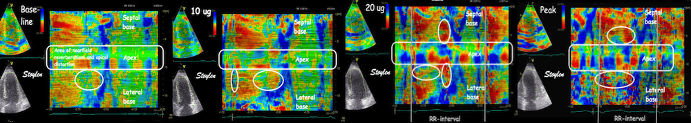
Thus initial delay of shortening (tardokinesia) has been seen as a component of ischemia from early experiments (177) as well as in late experimental (213) and semi-clinical (305) work. It is commonly used as a method for assessing B-mode WMS i stress echo (tardokinesia - 215)
In a totally passive segment, without any systolic shortening, the post systolic shortening may be simply passive recoil, as in the theoretical instance 5 above. However, even if there is holosystolic stretch, if the segment shortens more than it is stretched (instance 4), this is an indication of remaining tension, although too little to withstand the tension of healthy segments. This was demonstrated by Lyseggen et al (181).
And finally, if all segments have reduced function, the shortening pattern will be more normal Without any normal segments to interact with, there will in fact be less delay and no PSS, as shown by the following example where there is total ischemia, and hence, no normal segments and (almost) no PSS in the ischemic segments. Thus, the segmental pattern will be more normal, all segments have reduced contractility and delayed relaxation.
|
|
|
Severe ischemia in all walls in a patient with severe three vessel disease (among other things stenosis left main, occluded LAD filled from RDP, even with occluded RCA filled from collaterals) . Visually, the most striking finding is fall in EF with increasing stress. No segments have normal contraction, although the lateral wall is somewhat better then the septum | Strain rate colour M-mode. No significant PSS can be seen (Except possibly apicolaterally). Thus at first glance, the M-mode looks normal, at least concerning synchronicity. | Strain rate curves (top) and strain (bottom) of the ventricle at peak stress. Again, no significant PSS can be seen (Except possibly apicolaterally), demonstrating clearly that there are little PSS when there are no segments with normal contraction-relaxation cycles. The AVC is evident from the phono traces. The strain curves show delayed and prolonged shortening, but more or less in all segments. This is equivalent to the balanced ischemia of scintigraphy. |
The typical acute ischemic segmental pattern is thus:
|
|
The numerical assessment of systolic strain or strain rate, only considers one aspect of ischemic function, while the curve shape, or colur M-mode takes the whole time course into account, and thus gives more information, although qualitatively.
Small apical infarct.
|
|
The infarct shown above, with strain (left) and strain rate (right) curves from the septum, both showing that the apical segment has delayed onset of shortening (actually a little stretch before shortening), reduced end systolic strain (8%) and peak systolic strain rate (0.5 s-1), and post systolic shortening (additional 5% strain, and a new peak in strain rate). The basal segment (magenta) is normal both in shape and numbers, while tghe mid segment (orange) is in between. It is evident that the curve shape imparts far more information than the numbers. | Curved anatoimical M-mode, showing the time course of strain rate in colour coding. Colour M-mode is the qualitative strain rate - depth display, bt giving the same qualitative information as the curve display. |
Large, acute, apical infarct. The rocking motion is due to the uneven distribution of the infarct in the septum and the lateral wall.
|
|
|
|
Strain rate curves show a pattern that may at first look confusing, but the apical curve (orange), shows the most pronounced initial stretch (1), systolic hypokinesia (2) and post systolic shortening (3). All three segments in the sepotum are affected, but pathology is decreasing towards the base (magenta to white), where contraction (strain rate) is near normal, but the pattern is still pathological. The curved M-mode below shows the extent of the changes, numbes corresponfds to the phases shown above, initial stretch is blue, hypokinesia is seen by the dotted orange/green area (dotted because of thenoise in the signal), and near normal contraction and post systolic contraction is orange to red. | Strain curves from the same subject. The colours are reversed compared to the curves to the left, with white in the apex and orange in the base. Here, the apex is seen to stretch minimally through the whole systole, but close to zero (strain curves are smoothed compared to strain rate), while the curves shows increasing systolic shortening towards the base, but still with hypokinesia and PSS. Below is shown the theoretical curves corresponding. |
Comparing tissue Doppler and speckle tracking in the same infarct:

The midwall (magenta) curve in the left panel and the cyan curve in the right panel are from corresponding segments, showing basically the same curve shape. The scales on the TVI and speckle tracking are not equal.
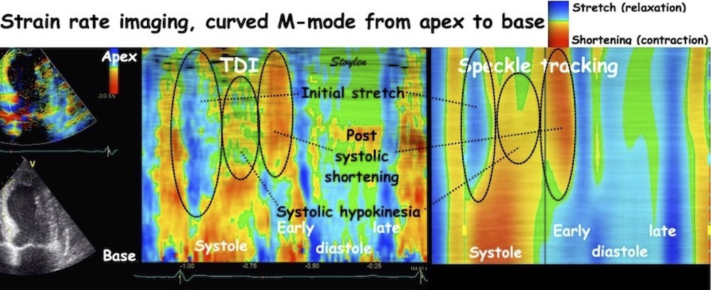
Curved M-mode from the same patient, comparing colour M-mode from TDI (left, and Speckle tracking (right), showing that the ST image seems smother due to the lower frame rate B-mode compared to tissue Doppler in addition to the spline smoothing of the 2D strain application. However, in this case, the resolution is sufficient to show intial stretch, apical hypokinesia and post systolic shortening also by 2D strain.
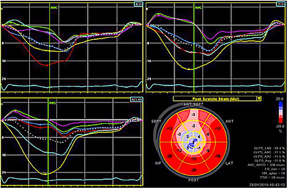
The same patient analysed with speckle tracking. The display bottom left is a bull's eye projection of the peak segmental systolic strain, with both numbers and colour codes. The three other panels show the segmentla curves from 4-chamber view (top left), 2-chamber view (top right) and apical long axis (bottom left). All views show systolic hypo- to dyskinesia with PSS in the apical part.
As shown above, in ischemia, post systolic shortening is caused by prolonged relaxation due to reduced activity of SERCA in ischemic (energy depleted) segments. However, it is important to realise that post systolic shortening is not only a phenomenon of ischemia, it can be seen both in left bundle branch block and hypertrophy. The mechanism is also in those cases asynchronous interaction between segments, but with different causes of asynchrony.
As discussed above, PSS in ischemia is only a part of a set of specific deformation changes in ischemia. As seen above, PSS is part of a complex change in deformation pattern, which is the delayed evolution of tension, reduced absolute tension and delayed relaxation in acute ischemic segments interacting with normal segments that causes the pattern of initial stretch, systolic hypo-, a-, or dys kinesia, with post systolic shortening. And without any normal segments to interact with, there will in fact be no PSS, as shown by the following example where there is total ischemia, and hence, no normal segments and (almost) no PSS in the ischemic segments.
Post systolic shortening (PSS) means that the segment continues shortening after the aortic valve closure, often after a short relaxation giving one or two peaks a systolic and a post systolic, or a single peak after AVC as shown in the figure below, left. The definition of shortening as post systolic is dependent on the location of AVC, which can be done by TDI as described above. This holds even in the presence of iskemia (with PSS) and in high HR (216).
|
|
|
Normal strain rate curves. Note that there is a little shortening of the lateral wall (cyan curve) after AVC (green vertical line). This is normal, and related to the shape change in IVR. | Initial systolic stretch, reduced systolic shortening and presence of post systolic shortening in the apical segment (cyan curve), with normal systolic shortening and no post systolic shortening in the basal segment (yellow curve). | Two different instances of post systolic shortening. Apicolaterally, there is stretching and then recoil after AVC (cyan curve), with possibly a little overshoot as indication of a remnant of tactive tension. Apicoseptally there is systolic shortening and then further post systolic shortening (yellow curve), which thus has to be active. It also shows the mechanism for PSS to be different than recoil. |
Already in the eighties, however, it was recognised that post systolic thickening and post systolic shortening was the same thing, due to the incompressibility as discussed above, and that the PSS in acute ischemia was a marker of active tension.
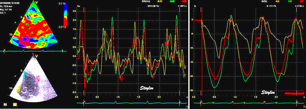
Inferior infarct (yellow), showing both reduced strain rate and strain, with shortening after the normal shortening of the healthy segments (post systolic shortening). In this case, there is both systolic (although reduced) and post systolic shortening, thus the PSS has to be due to active tension, as in instance 2 above.
The presence of PSS in acute ischemia in the clinic was shown with M-mode by Henein (217), and later with strain rate by Jamal in 1999 (218) and Kukulski (199, 200).
Post systolic shortening has been proposed to an additional diagnostic criterion for ischemia in stress echo, but larger studies has not shown additional diagnostic value of this (219).
As seen by the colour M-mode below, the presence of post systolic shortening in a segment, leads to a delay in the onset of segmental lengthening compared to the normal segments, so the finding is equivalent to the delayed compression/expansion crossover described by some authors (220).
Post systolic shortening is usually visible both in tissue velocities and in strain / strain rate, but for location of the phenomenon (and thus ischemia), deformation imaging is best.
| |
Apical myocardial infarct in the inferolateral wall. Inward motion after systole can be seen in the apex. | In this case we see systolic stretch in the apex, and with PSS as in instance 4 above, midwall initial stratch and then systolic shortening with further PSS as in instances 2 and 3 above, and then normal shortening and relaxation in the base. That post systolic shortening in the infarct area is simultaneous with elongation (relaxation) in the normal basal part, is very evident from the colour M-mode. |
| |
Looking at tissue Doppler, there is post systolic motion of the borders of the midwall segment (lilac and orange curves), but very little in the apex (green) or the mitral annulus (white). | But this of course means that post systolic deformation happens in the apical segment (yellow coloured interval between green and orange curve). |
|
|
The post systolic shortening is thus in the infarcted apical segment (yellow cirve, negative deflection) as seen from the strain rate ..... | .... and strain curves. |
Also, comparing strain and strain rate curves, with the velocities, it can be seen that post systolic shortening only reslts in relative motion, without much over all effect on the motion of the mitral ring.
Post systolic shortening can also be seen to affect flow directly, actually no surprise, but this was described early in an observational study (365) before the concept of PSS was fully described.
As in the example above, the area of a- to dyskinesia is the area most affected by ischemia (instance 4 -5 above), while the surrounding area will have systolic and post systolic shortening as in instance 2 - 3 aboveshowing a lesser degree of ischemia. 3D starin rate mapping will show this, the area of dyskinesia being smaller than the area of PSS:
| |
Strain rate bull's eye and three dimensional reconstructions of a ventricle in systole (top), showing an area of dyskinesia (blue) in the apex, and diastole (bottom), showing a larger area of post systolic shortening (yellow). | Strain rate bulls eye from systole and early diastole (top, left) , below 3D reconstruction (bottom, left) in systole and M-modes from all six walls (right), showing an inferior infarct with slight dyskinesia and more extensive akinesia in systole and post systolic shortening in a larger area also around the infarcted wall. |
Presence of ischemic PSS may give asynchrony between walls, where almost all of the wall may be out of phase, even if there are gradients of ischemia as shown below.
|
Stress echocardiography with development of ischemia in the inferolateral wall. At peak stress, the whole of the wall can be seen to move paradoxically, moving inwards (and towards the apex) after end of septal contraction. Again, in a clinical situation, the interpretation can be facilitated by stopping and scrolling. |
|
|
The velocity (motion) confirms the visual impression, the whole inferolateral wall moves downwards in systole, and upwards after end systole (Yellow and green curves), while the septum shows normal apically directed velocities giving a total asynchrony between the two walls. This asynchrony is also evident by the curved M-mode, starting a the inferior base, going through the apex and ending at the septal base.This might be due to both apical and basal ischemia. | |
|
|
The strain curves below, separates the effects of the segments, showing systolic dyskinesia (lengthening) with some net post systolic shortening in addition to the recoil in the base (yellow curve), and systolic hypokinesia in the apical segment (green curve) with post systolic shortening, compared to a fairly normal strain curve in the septum. Thus, deformation imaging showing most severe ischemic reaction in the basal part, giving highest probability of a Cx ischemia, which was confirmed angiographically. | |
In this case, the tissue velocities are sufficient to detect the presence of ischemia, but the deformation imaging shows the location and extent of the ischemia, while velocities shows asynchrony of the whole inferolateral wall. Thus, the basolateral ischemia might have been mis interpreted for lateral asynchronia.
The presence of regional systolic dysfunction in combination with post systolic shortening, may cause asynchronous motion of a whole wall, as shown above. This means that the presence of asynchrony in motion imaging is not specific. A further example, also from stress echo; i.e. ischemia, is shown below.
|
|
3D colour velocity images showing motion towards the apex in red, away from apex in blue. Left, systolic 3D reconstructed image, showing normal motion in the septum and inferior wall, and paradoxical motion in the inferolateral, lateral and anterior wall. Right, om top are bull's eye from systole, showing the same, as well as early diastole showing inverse motion during the e-phase, i. e motion of the whole wall towards the apex in diastole. Apparently, the whole anterolateral half of the ventricle is ischemic . | 3D strain rate images from the same recording, left systole, right early diastole, showing that the ischemia is due to a smaller ischemic area in the inferolateral, lateral and anterior apex, where there is streching during systole (blue). This stretching, results in the midwall and basal segments moving away from the apex, despite contracting normally. In early diastole there is recoil in the ischemic area (yellow), resulting in anterior diastolic motion in the whole of the wall. In this case, the ischemia is obviously limited to a part of the apex, the rest of the motion abnormalities being due to tethering. |
In acute ischemia, the prolonged tension / delayed relaxation is due to a reduced rate of removal of cytoplasmic calcium due to energy depletion. As shown in experimental ischemia, as well as in PCI studies, this reverses quickly with normalisation of flow ( 198 - 201, ). However, longer duration of ischemia, or repeated ischemia will lead to a prolonger stunning of the myocardium, affecting both contraction and relaxation (202). The mechanism of PSS is prolonged relaxation due to lack of energy affecting the SERCA in ischemia or in prolonged stunning, in interaction with normal functioning segments. Thus normalisation of systolic function would be expected to be paralleled by a reduction of PSS, as seen above (182).
Studies have shown that stunning in the acute phase of an infarct mainly recovers during the first 1 - 2 days (182, 183, 203). Thus reduced systolic function seen later would be permanent (loss of myocytes / scarring). PSS decreased concomitant with increase in systolic function. The post systolic shortening was about the same in border zone segments and infarct segments, despite infarct segments having lower absolute value of peak systolic strain rate. The PSS diappeared in the border zone segments in a week, but continued to decrease somewhat in the infarcted segments during a longer observation period (182), indicating that the diastolic stunning might last somewhat longer. However, some PSS remained also after 3 months.
In a cross sectional study (204) Voigt et al found PSS to be present in normals as well as infarcted hearts, in normals it was present in up to about 30% of segments, but then associated with normal systolic strain, and being both less in magnitude and earlier in the peak than in infarcted segments. It was present both in acute infarctions and in chronic infarcts. In acute infarcts, it was seen in 78% of ischemic segments, in older infarcts in 79% of scarred segments (which may presumably be fewer than in acute ischemia). Thus, the ischemic relaxation dysfunction is not the only explanation for PSS.
Loss of longitudinal fibres in myocardial infarction (186) will lead to loss of contractile force in the longitudinal direction. This is equivalent to a local increase in the load/contractility relation. Thus, reduced muscle mass will result in increased relative load from healthy segments, and this alone may be a mechanism for delayed relaxation in affected segments (179), although without the additional delay from hypoxia. So, the PSS in infarcts would be expected to decrease in magnitude with time.
|
|
|
|
|
|
Small acute apical infarct showing delayed onset of shortening, hypokinesia and post systolic shortening in the apicoseptal segment. | Same infarct 1 month after successful revascularisation of LAD, apical delayed shortening have disappeared, syst strain rate have increased some, and the PSS have decreased both in amplitude and extent. |
Increased fibrosis may reduce the systolic stretch in the infarcted segments, even if the segments remains weakened, and reduced stretch will also give reduced recoil. A weakened segment will have increased relative load, as peak tension is lower, which is another mechanism for delayed relaxation.
|
|
|
|
|
|
Large apical infarct in the acute phase. Initial stretch (1), pronounced apical and midwall hypokinesia (2) and pronounced PSS (3). | Same infarct after 3 months. There's no longer initial stretch, despite pronounced apical hypokinesia, indicating, increased fibrosis, still apical and midwall PSS, but less in magnitude. |
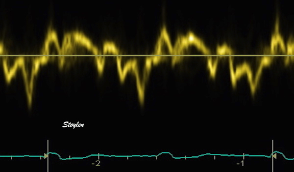
Typical pattern of tissue velocity in the septal base, in a case where LBBB induces mechanical asynchrony.
left bundle branch block may have very different mechanical effects. This is due to the very large variability in how much, and which parts of the left bundle that are affected, and to what degree.
Basically, left bundle branch block means a reduced conduction velocity in the left bundle, below that of the right bundle, causing the septum activation direction to shift from left-right to right-left, but also meaning that parts of the left ventricle are activated later than the right, and later than normal, causing a widening of the QRS. The mechanical effects of the LBBB may be quite various, however:
Thus, the mechanical manifestations are various:
The bundle branch block may cause
The pattern of deformation in left bundle branch block is also due to interaqction between walls, as they interact differently when the activation sequence interact.
If there is intraventricular asynchrony, this is usually very evident, and the most typical marker is the "septal flash".
The most typical pattern, originally called "septal beaking"(as it was origially described in M-mode), was described early (205). Later, it has been termed "septal flash" (206).
"Septal beaking" in M-mode; a short inward motion starting at the peak of QRS, and peaking at the same time as the onset of inward motion of the inferolateral wall. The contraction of the lateral wall is the force terminating the septal flash, so the time from onset of septal flash to onset of inferolateral wall thickening is the true mechanical delay between the walls. | Septal flash seen by B-mode in the same patient. The septal flash consists of a short inward and then outward motion of the septum, the outward motion start about simultaneously with inward motion of the lateral wall. The "septal flash" is evident in both parasternal long axis and short axis. Images from patient with normal systolic function. |
The isolated contraction of the septum probably will not generate pressure increase, but rather stretching of the lateral wall as seen by strain rate and apical rocking. During septal tension, the start of lateral wall contraction will generate pressure increase, which can be seen by the trasverse outward motion after the inward peak.
What we see is a pattern of septal flash, shortening during ejection, late systolic stretch and post systolic shortening.
Typical pattern of tissue velocity in the septal base, in a case where LBBB induces mechanical asynchrony. The septal flash can be seen early, then the ejection, then late systolic stretch of the septum, which is due to the continuing tension in the lateral wall (being delayed), and then post systolic shortening of the septum due to recoil from the previous stretch, simultaneous with the relaxation of the lateral wall.. | The M-mode shows the same. (Another patient, but the pattern is similar). The septal inward motion starts early during QRS (first vertical line). The peak is when the lateral wall thickening starts (second yellow line). During lateral wall thickening there is much less thickening of the septum, which actually seem to move outwards. Then at peak lateral wall thickness (i.e. when lateral wall starts thinning), inward motion and thickening of the septum starts again (third yellow line - post systolic thickening) and then peak septal thickening is simultaneous with the end of the steepest part of lateral wall thinning. |
The complex motion pattern in the septum must be explained by the interaction between the walls:
|
|
|
|
|
Septal activation alone. leading to septal shortening and thickening, with concomitant lateral stretch - the septal flash. No pressure increase. | Lateral wall activation, ending the septal flash which peaks) with remaining septal tension (or else there would be only rocking, no pumping). In this case there is pressure buildup, MVC, IVC and probably start ejection. | During most of the ejection there will be shortening, but part of this may be passive due to volume decrease, especially in the septum. | In the last end of the ejection there will be little or no remaining tension in the septum, which then will stretch, due to the remaining tension in the lateral wall (which have been activated later). Thus, there will be stretch og the septum and shortening of the lateral wall. | Finally, there is no tension in the lateral wall, which relaxes. In this phase there will be elastic tension in the septum due to the previous stretch, which will shorten in post systolic shortening, while the lateral wall stretches (both due to septal shortening, but also in the course of normal early filling). |
The phases wall interactions above, visualised in colour SRI.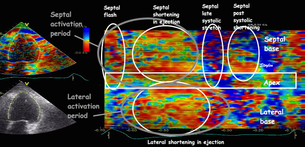
The pattern from the septum in the TDI above can be seen in this SRI M-mode. But here the phases being result of interaction between the asynchronous walls is more visible.
Comparing the tissue velocity curves with the strain rate CMM:
The different timing of the two walls is evident in the tissue Doppler tracing from the base of the same patient with normal ventricle. The action of the two walls can be inferred from the ring motion, and the interaction as one wall or the other is active while the other is passive, explains the complex pattern seen in the tissue Doppler above. This raises the question, which is the septal e' wave? The late systolic septal stretch, is the septal relaxation, but firstly, is mainly introduced by lateral contraction, and secondly, do not occur during filling. The post systolic shortening, is closest to the early filling, but is actually an impediment to the filling itself. | The strain rate from the same pateient shows this more directly, illustrating the simultaneous stretching of one wall and shortening of the other. We also see differences in timing between base and apex both in septum and the lateral wall. |
Of course, this septum - free wall interaction depends on the normal function of the LV lateral wall, with lateral dysfunction, the typical pattern doesn't appear (217). On the other hand, the LBBB seems to offload the RV, so CRT may be deøeterious for patients with RV dysfunction (218).
LBBB also affects the diastolic function, by causing asynchronous e' between septum and lateral wall:
The problems of defining e' is evident, while the late stretch is the true relaxation of the septum, it is not due to only relaxation, being facilitated by the simultaneous lateral contraction, the post systolic shortening is closer to, and dependent on the relaxation of the lateral wall, but as the relaxation of the lateral wall is taken up by the septal recoil, it does not generate so much suction into the ventricle (and the post systolic shortening may be seen as opposing filling. Thus, mitral inflow is seen to start late, and showing a low E/A ratio, which, however is mostly due to EA fusion.
The septal flash is the equivalent to the "rocking apex" (207) also described in LBBB, as the asynchrony induces a rocking motion of the apex as seen in the four chamber view. The rocking apex is due to the initial contraction of the septum without simultaneous contraction in the lateral wall that results in the rocking towards the septum. The rocking due to septal flash, is always toward the septum, while the rocking apexes shown where the whole heart rock (not due to conduction anomalies), is more often towards the lateral wall. The rocking is also evident in the tissue Doppler images, although with a complex pattern:
| |
The four chamber view shows both septal flash and rocking apex, but the initial rocking is towards the septum, and the septal flas is simultaneous, the blater rocking towards the lateral side ios concomitant with the bcontraction in the lateral wall. | "Rocking apex" as seen by tissue Doppler. The apex moves first towards the left. This is evident as the left side of the apex moves downwards (yellow curve - initial downward velocity) and the right side moves upwards (cyan curve, initial positive velocity). After this initial rocking, the apex stays in the new position for a period as seen by the two curves lying close together. the there is slow motion towards the lateral wall, and then an abrupt reverse rocking (negative cyan peak - downwards motion of the lateral apexand positive yellow peak - upwards motion of the septal apex). Finally, there is even another reverse of the rocking after end systole, due to the post systolic septal shortening described above. |
However, looking at the B-mode above, the motion is far more complex than this. The initial inwards motion of the septum is reversed, the rocking of the apex towards the septum, however is not reversed before mid systole, where the apex rocks back.
|
|
|
The ejection period timed by Doppler flow from LVOT. | The phases are visible by tissue Doppler. This is the same image as above, but with two more sample volumes added in the base. (the differences in amplitude of the apical curves is due to autoscaling). Deformation is visible by the offset between the velocity curves; there is septal shortening when the red line lies above the yellow, and lengthening when yellow is above the red. Likewise in the lateral wall there is shortening with green above cyan, and lengthening with cyan above green. During QRS there is shortening of the septum (yellow to red), and stretching of the lateral wall (green to cyan). This is the septal flash. With onset of lateral shortening, the septal flash reverses, resulting in the peak of the septal flash (yellow vertical line), which also marks the MVC and onset of IVC. At start ejection, there is abrupt apical velocities of both basal points, marking shortening of the whole ventricle, as seen by the velocity offset, there is shortening in both septum and lateral wall. before end ejection, however, the septum starts to stretch due to end of relaxation, as seen by the yellow/red crossover. This continues after end ejection, while the end of lateral shortening is marked by the cyan green crossover, also marking the onset of post systolic septal shortening. | The findings from tissue Doppler is confirmed by this curved M-mode, showing the phases of septal shortening and lateral stretch. The peak of septal flash is the shift from septal shortening to elongation, concomitant with the onset of lateral shortening, although in this case it is difficult to discern because of noise. The yellow marker have been carried over from the previous image with tissue Doppler curve. |
Thus, mechanical asynchrony in LBBB can be diagnosed by the septal flash or the rocking apex, but NOT necessarily by time to peak systolic velocity.
Finally, there will be relaxation of the lateral wall, when this is passive, there will be elastic tension in the septum, and it will recoil in a post systolic shortening (E).
However, it is important to realise that the septal flash (and indeed the rest of the mechanical asynchrony) can be seen in ventricles with good function as the above instance. The septal flash is thus a marker of asynchrony, but not necessarily to a degree leaading to heart failure. In the above case, there is evidence of some mechanical inefficiency, as there is end ejection shortening of the lateral wall and stretch of the septum, with stretch of the septum and some recoil (post systolic shortening) which may indicate "wasted work". However in this case, most of the rocking happens after end ejection, there seems to be little wasted work during ejection.
The asynchrony, may still be a marker of some degree of mechanical inefficiency, But this may not become important unless there is underlying myocardial disease with weakened myocardium from other causes as well. However, this may also be dependent on the degree of delay of the lateral wall. It cannot, however be any doubt that the deleterious effect on mechanincs which may be improved by CRT, has to be through mechanical asynchrony.
The width of the QRS, however, even if being statistically associated with prognosis, may not be an individual marker of the degree of asynchrony. The QRS width is a marker of the amount of delay, but not where the delay is situated, and thus says less about mechanics.
Septal flash is a marker of mechanical asynchrony per se, but not necessarily of mechanical inefficiency. Thus mechanical asynchrony may be necessary, but not sufficient prerequisite for assuming that the patient suffers from mechanical inefficiency.
As CRT now has been a well established treatment modality for heart failure with Left Bundle Branch Block (208 - 210), much interest has been vested in eliciting how mechanical asnchrony may affect pumping efficiency. It seems that the mechanism may in many cases be through mechanical inefficiency, due to asynchronous work by the left ventricle. The septal contraction without opposing tension in the lateral wall, and thus without ejection may be considered wasted work. However, as many ventricles with normal function and LBBB doesn't have HF, this may not matter if there is no basic myocardial failure underneath.
Resynchronization may result in improvement due to more efficient work.
As only about 70% of CHF patients with LBBB respond to cardiac resynchronisation therapy (CRT), the need to elicit the effect on mechanics in order to see which patients that are potential resonders, seems obvious. However, so far, the search for echocardiographic markers of mechanical inefficiency that may predict response, have only beeen moderately successful (211). It may be that in some patients the LBBB is a marker of cardiac disease, without being a worsening factor.
Of course, simplistic approaches such as using dispersion of "time to peak systolic velocity" would be far too simple. Especially, as the peak systolic velocity is not a function of electrical activation, but of peak ejection velocity after AVO. "Time to peak strain rate" is largely the same, the peak rate of shortening, but not only of AVO, but also the rate of force development. Uneven contractility would thus be expected to be a factor in timing of peak deformation rate.
Septal flash is a marker of mechanical asynchrony per se, but not necessarily of mechanical inefficiency.
The concept of "wasted work" describing mechanical inefficiency has been suggested (194) as a description of how the work of shortening in one segment leads to stretching in another, instead of resulting in ejection. The concept may be fruitful, as it indicates that much of the work in shortening parts of the ventricle do not contribute to ejection work, but instead stretches another part of the wall, and is thus " wasted", and which is potentially recruitable by CRT.
However, it is unclear what adding a global systolic pressure measure will add, compared to just looking at net strain in opposing walls (212): The shortening of one wall and simultaneous stretch of the opposing wall, called "simple regional strain analysis" seems to approach the same concept of wasted work, and is promising in being a marker of potential response to CRT. As the difference between segments are only the strain, while the pressure curve is the same, only the strain carries the information of the differences in regional function. Thus, this is actually the Emperor's new clothes. And the method will be just as sensitive to noise, as regional strain, of course.
Top left: strain pressure loops in a patient with LBBB. It's the same patient as above. Top right, the pressure curve. Bottom, strain traces. The strain-pressure loops are generated by plotting the strain traces against the pressure curve, but as the pressure curve is the same for both walls, the differences between the loops are only due to the differences between the strain curves, and the wasted work is the work when one wall shortens while the other stretches, basically in early systole (septal flash - 1) and in end systole (after 2).
However, the approach by only looking at total strain may be too simplistic, and so may integrating it into a simple index.
Mechanical inefficiency may be more evident in the next case:
|
| |
There is septal beaking in the M-mode, start of the septal beak is slightly after start of QRS, septal peak is about simultaneous with onset of inferolateral thickening, and then there is a slight septal inward motion simultaneous with the inferolateral wall thinning and finally onset of post systolic thickening at the peak of lateral wall thickness (onset of thinning). | Septal flash is evident form the parasternal view. | And both septal flash and rocking apex in the apical 4-chamber view. |
|
|
Looking at apical velocities, the apical rocking to the left during septal activation (A - C) is evident, while there is a period with little rocking, and then rocking to the right during the last part of systole (E-F). | Adding basal curves (again the apical curves are the same, amplitude is only due to autoscaling), it is easy to see septal shortening and lateral stretch during the septal flash, with the peak (B) more or less at the same time as in the M-mode. |
Looking at strain rate, the same can be seen, both in the M-mode and the traces, there is septal shortening and lateral stretch from A to C. The peak of the septal flash (B) is not easily seen in colour M-mode, but must more or less correspond to the onset of lateral contraction (tension), which is the force (through increasing pressure) that forces the septum back. | |
|
|
Finally, looking at true ejection, it can be seen to start at (or even slightly after) the end of the septal flash, indicating that IVC occurs during the last part of the flash (probably from the peak). But ejection is still during lateral wall shortening. | This is partly confirmed in the mitral flow curve, the end of flow and mitral valve closure as seen by the valve click, occurs at nadir QRS, nearly simultaneous with peak septal flash, indicating that IVC starts at that point. |
In this case, there is evidently more asynchrony, as well as indications of less energetical function more wasrted work), as more of the systolic time seems to be used for stretching of opposite walls. The differences may be due to more delay in electrical activating the lateral wall. However, the QRS width is not a good indicator of this, as the factor here logically will be onset of lateral activation, not end.
Ejection fraction is also lower in this case (The patient has had mitral annuloplasty, and preoperative dilatation due to MR), but it will be difficult to ascertain whether the function is reduced due to worse electrical asynchrony, or the mechanical asynchrony is worse due to a reduced ventricular function. However, in this case there may be potential for recruiting more contractility by CRT, and the patient may be candidate for CRT if developing manifest CHF.
The main consequences of this mechanics, is that the lateral wall does most of both pressure and ejection work, and thus less muscle is recruited for work. In the case of a weakened ventricle, at least, the reduced global force and wasted work force will tend to worsen the function.
The mechanics may be far more complex than this, as in the next case:
|
|
Apical rocking (equivalent with septal flash can be seen by tissue velocity curves in the apex. | |
| |
Looking at another example, cardiomyopathy with CHF, LBBB and septal flash, asynchrony is evident, even without tissue Doppler. | Adding the velocity curves from the base shows very little dyssynchrony assessed by the time to peak annulus velocity, in fact by that criterion it seems fairly synchronous. Also, assessing the strain rate by the offset between the velocity curves (septum yellow and red, lateral wall cyan and green), there seems to be a fair strain rate in both walls. |
|
|
Although the septal flash, with septal shortening and lateral stretch is visible (before the red marker line), surprisingly, in this case there seems to be more shortening in the midwall septum than the lateral wall, both in strain rate, | and strain.This seems to be counter intuitive as the mechanical inefficiency is a function of septum contracting before lateral wall, which the does most of the real work. |
|
|
Looking at the velocity curves from apex, midwall and base, the points in each wall seems to be fairly synchronous, but the offset between the curves from neighboring points are variable. | In the septum, the offset between the apical curve and the midweall curve (strong orange) is greater than between the midwall and basal (strong green), where there even are some periods of systolic stretch weak green). |
|
|
Strain rate curves from the segments between the curves to the left, shows shortening in the basal half (orange), while the septal half (green) has stretch, slight shortening and then stretch again during ejection. | In the lateral wall the situation is opposite, there is very little shortening, and even a little systolic stretch in the basal half, and better shortening in the apical half. |
This is even more evident in the colour M-mode:
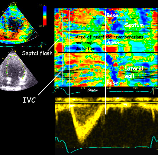
Vigorous systolic shortening in the basal part of the septum and apical part of the lateral wall, less so in the apical septum and lateral wall, systolic stretch being most evident apicoseptally.
This dissociation between the apical and basal parts may be the reason for the apparent dyssynchrony when assessed by the apical velocities (rocking apex), and the far less dyssynchrony evodent in the basal velocity curves.
However, in this case there is just as much asynchrony and wasted work (corresponding to one whole wall, but distributed between the two walls), not located in one wall only. However, with evidence of mechanical inefficiency, it is not surprising that the patient responded very well to CRT:
|
|
The response after 1 year shows reverse remodelling, increased EF, and abolished septal flash. | The same is evident from the apical view. |
| |
And synchronicity of shortening can be seen by strain rate. | |
Finally, looking at an extreme example:
Dilated cardiomyopathy with left bundle branch block. Early contraction of the septum with short duration (septal flash and apical rocking) is visible, and there is delayed contraction of the lateral wall. The septum is thinner than the lateral wall, which may indicate that only the lateral wall carries load. | Looking at the strain rate colour M-mode, the same is evident, even despite the heavy reverberations in the lateral wall. In this case the septal flash represents the whole of the septal shortening, with simultaneous lateral stretch. Septal stretch is evident during most of the main lateral wall shortening. In this case, however, it can be seen that the most vigorous (rapid) lateral shortening starts before ejection, because the pressure buildup (IVC) has to be done by the lateral wall while some of the work already during this phase is wasted by stretching the septum. |
|
|
Looking at the ejection, it can be seen to start during the period of the most vigorous lateral shortening, and then persist during the phase of bilateral shortening. The ejection phase is abbreviated. | End of mitral flow (MVC) can be seen just before the peak of the septal flash on the M-mode to the left. There is also E-A fusion, at normal heart rate, indicating an AV-block. In this case the PQ time is normal, but there is a functional block to the left ventricle due to the bundle branch block. |
Looking at strain rate curves, the information is the same as the colur M-mode above. Start ejection is marked by the white line. We see that the most vigorous lateral wall shortening occurs before start ejection, and is balanced by septal stretch. This represents isovolumic contraction period, but as can be seen from the curves, much of the work seems to be wasted on stretching the septum instead. There is little shortening during the ejection period itself. Finally, there is post systolic shortening, but this is after end ejection. | The mechanics may be more intuitive by strain than by strain rate, when looking at the traces, showing a brief shortening of the septum (septal flash), and then stretch. The ejection is again seen to start after the most vigorous lateral wall shortening, indicating that much of the work during IVC goes into stretchingthe septum. During ejection there is a slow decrease in septal stretch (i.e. a little shortening, and a greater stretch in the lateral wall. After ejection there is reversal of lateral shortening and septal stretch (post systolic shortening). |
In this case, the unfavourable mechanics is even more evident, but to understand it fully, there has to be a comprehensive evaluation. As so much of the work seems to be wasted, there are indications that CRT might result in improvementby recruiting the septum for active pumping work.
This proved to be the case:
The same patient 6 months after CRT. Reverse remodeling and increased EF is evident. Now, the septal flash can no longer be seen, although the overall motion is not completely normal, in fact the apical rocking has reversed, there is now an inverse rocking to the right at early systole. Also, the septum has thickened as a response to carrying more load. | Now, there is early shortening of both walls during pre ejection, ending with MVC as seen below. During the whole of ejection there is simultaneous shortening of both walls. |
|
|
Ejection is earlier, compered to ECG, as is IVC, and the ejection period is longer. | However, there is still E/A fusion, indicating an AV-block to the left ventricle, so the CRT may not be completely optimised. |
However, the strain rate curves look much more normal as well as synchronised. In fact, the lateral wall seems to activate slightly before the septum. | This is also evident from the strain curves, both wall shortens simultaneously, although the onset is earliest in the lateral wall. And looking at the programming, the lateral wall was actually programmed 40 ms before the septum. |
In this case, not only the mechanics due to the LBBB, but also the deleterious hemodynamic consequences of the asynchrony, as well as the sucessful recruiting of the septum for pumping work, was evident.
Tissue velocities on the other hand did not contribute to the understanding, neither before or after CRT:
| |
Looking at velocities, there sis an earlier peak velocity in the septum than the lateral wall, indicating asynchrony although not very much more than the previous case when looking at peak velocities). The mechanics is not evident from this image, especially as this shows higher velocities in the septum. | It is not very evident from the tissue velocities image that the left ventricle has been resynchronised. |
However, this could only be demonstrated, by a comprehensive analysis of mechanics and hemodynamics. Also, the cardiomyopathy may still be the cause, and the LBBB only the worsening factor, creating a viciuous circle. (That LBBB was truly a worsening factor, was actually demonstrated by the improvement after CRT.
It seems that echocardiography, especially deformation imaging, can go a long way in describing the mechanics in bundle branch block, and may also indicate if there is potential for CRT by describing "wasted work", but it seems that this needs a comprehensive evaluation of both mechanics and hemodynamics. Simple indexes of mechanical asynchrony, such as time to peak velocity, time to peak strain, or even septal flash or rocking apex (as these may be present without very poor mechanical performance). Also, of course, intraventricular mechanics may not be the only factor in predicting CRT response.
This, of course is bad news for large scale studies looking for simple echo criteria / indexes that may predict CRT response, in the words of the PROSPECT investigators: no single echocardiographic measure of dyssynchrony may be recommended to improve patient selection for CRT beyond current guidelines (286).
Multivariate analysis may still show factors positively associated by response, but a comprehensive hemodynamical analysis should be worked into a scoring system, if it is to be evaluated.
Pacing is commonly done by a transvenous lead into the right ventricle. For reasons of safet, it is often placed in the RV apex, to minimise the risk of lead displacement. This however, means that the initial activation may be in the right ventricle, also activating the septum before the lateral LV wall, analoguous with the LBBB. (In fact RV pacing is LBBB). But the lead placement may give differente effects, especially the efect in the apex vs. the base.
| |||||||||
|
Mechanical dyssynchrony seen by tissue velocities and strain rate and strain, all from the same heart cycle. The phases during systole are shown with the letters corresponding to the diagrams above. Valve closures and openings are marked on Doppler flow recordings, and transferred to the present loop. The apical rocking during phase A is evident from the apical velocity tracings. The action of the two walls can be inferred from the ring motion, and the interaction as one wall or the other is active while the other is passive, explains the complex pattern seen in the tissue Doppler above. This raises the question, which is the septal e' wave? The late systolic septal stretch, is the septal relaxation, but firstly, is mainly introduced by lateral contraction, and secondly, do not occur during filling. In fact, the relaxation of the lateral wall is seen to be absorbed by the septal PSS, before MVO, which is delayed. Thus the active LV seuction is abolished. The post systolic shortening, is closest to the early filling, but is actually an impediment to the filling itself. The strain rate from the same patient shows this more directly, illustrating the simultaneous stretching of one wall and shortening of the other.