Amount
and method for temporal averaging should always
be reported in clinical studies.
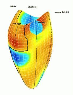
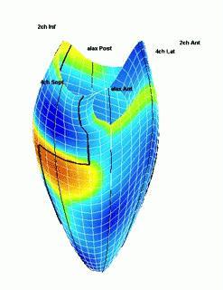
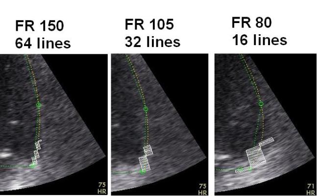
Insonation
angle deviation in different parts of the
ventricle_
 |
 |
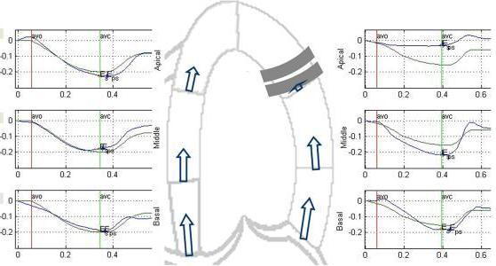
Which
segment that is most in alignment with
the ultrasound beam, may vary
with LV depth as illustrated
here.
|
 |
LV shape also is important in
determining the degree of wall alignment.
|
It has been
maintained that strain and strain rate
cannot be measured in the apical segments,
but from the illustrations shown above, this
is not necessarily true for all patients on
a segmental level, and the apical segments
may in fact be the ones showing best
alignment in some cases.
However, the apex seems most susceptible in
the
HUNT study, but
the problem was solved by the ROI tracking the
myocardial motion.
In post processing, the main
point is to exclude segments with to
great angle deviation from analysis, at
least other than timing by parametric
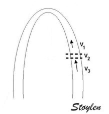
In some instances the angle problem is due to
imperfect alignment (foreshortening), if the
probe is not positioned properly over the
apex. (As indeed may be necessary to obtain an
acceptable window). In that case, the angle
problem can vary along the wall as shown
below:
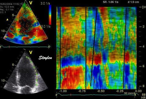
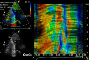
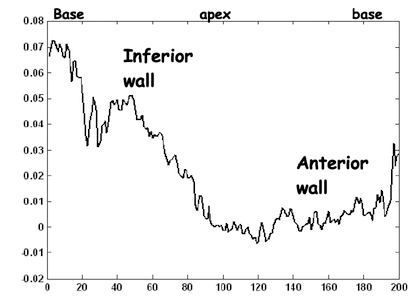
Less
than perfect alignment with the
apex, results in a, angle along
the inferior wall in this
2-chamber view. It can be seen
that the wall apparently is
curved, and that the alignment
is better in the basal than the
apical half.
|
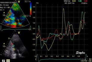
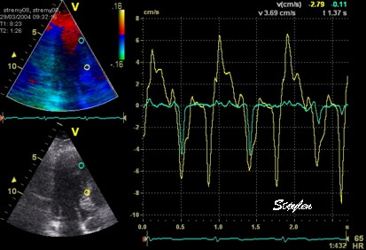
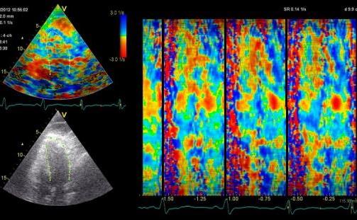
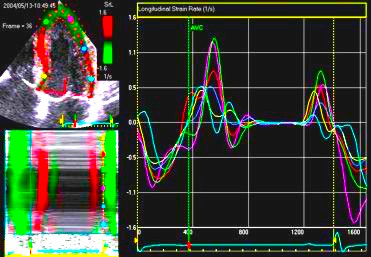
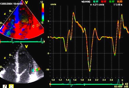
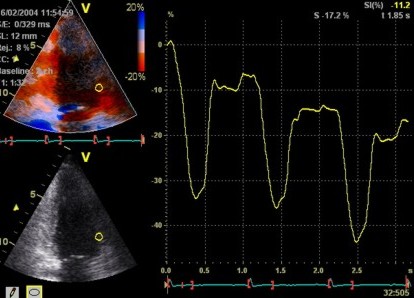
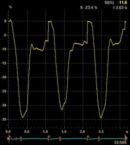
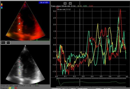
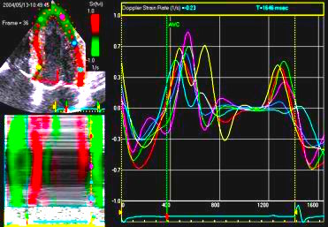
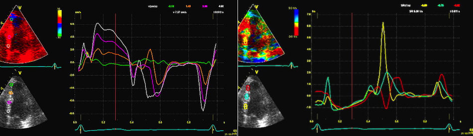
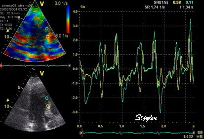
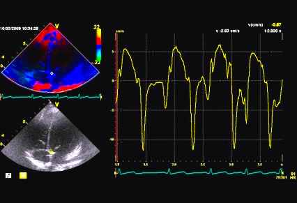
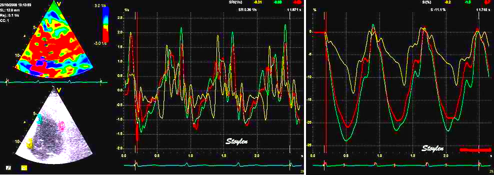
This
has different effect in the
different parts. Basally, there is
a normal strain rate curve
(yellow). Apically, the systolic
strain rate is reduced to half,
due to angle distortion (red). In
the midwall, there is a normal
peak value, but the systolic curve
is cut off, resulting in zero
values in the late systole (cyan).
as the bent area moves into the
ROI.
|
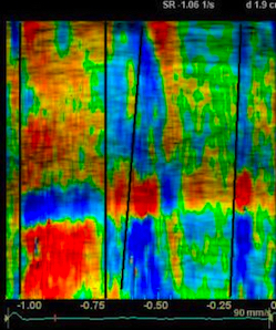
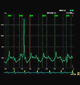
This
is also apparent in the curved
M-mode, showing an area of apparent
a- to dyskinesia in late systole in
the midwall.
|
Using timing information, especially the
shifts between positive and negative strain
rate, on the other hand has been proposed to
overcome the angle limitation. This, however,
may be problematic if the alignment is less
than perfect, in a way tat the angle between
the ultrasound beam and the wall varies
through the heart cycle, as shown in the
midwall segment in the middle image above.
Variable
insonation
angle during the heart cycle
In individual cases, there may also be angle
problems in other levels, especially the
inferior wall in the care of foreshortening.
The angle deviation may apparently vary during
the heart cycle.
 |
 |
|
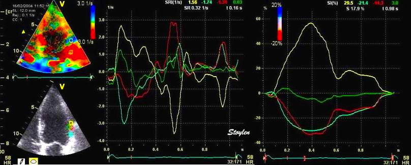
| Two
chamber view. The apex is in fact
outside the sector to the left,
and the inferior wall appears to
have a break in the midwall. |
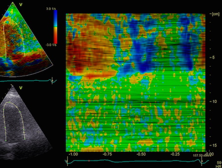
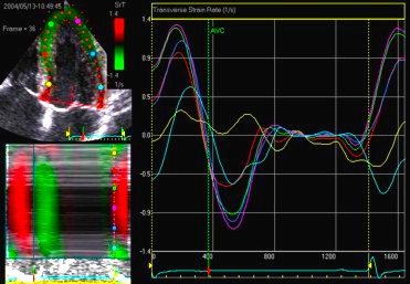
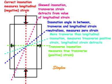
The
middle part is transverse to the
ultrasound beam, and here the
measured strain rate will be wall
thickening (positive strain rate),
as shown in the diagram,
longitudinal shortening (negative
strain rate; orange arrows) in the
apex and base, transverste
thickening in the midwall
(positive strain rate; cyan
arrow). |
In the
curved M-mode, the area of
positive strain (transverse
thickening is seen to move with
the wall. The pattern may resemble
a reverberation, but doesn't last
throughout the heart cycle, and
the time course is not horizontal. |
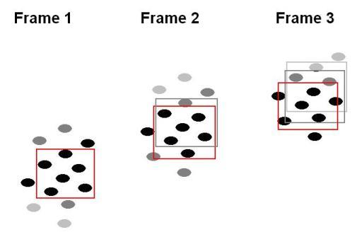
The motion of
the distortion area suggests how to deal
with this artefact by making the ROI track
the myocardial motion, as shown here.
Tracking
the ROI:
Commercial software have the option of
tracking the ROI manually, but the tracking
could be done by automatic methods as in the
NTNU application.
The tracking eliminated the systematic angle
problem in the apex in the HUNT study.
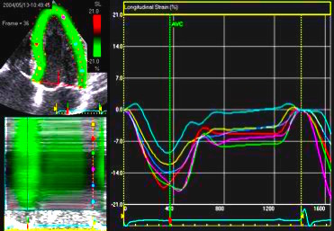
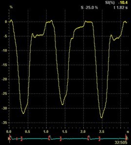
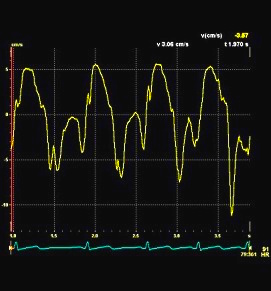
The
same loop as above, showing normal
strain rate curve in the base
(yellow), but abbreviated systolic
strain rate curve in the midwall,
as the area of transverse strain
moves into the ROI.
|
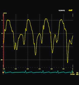
The
same ROI placement in start
systole as left, but now the
ROIs are made to track the
myocardial motion through
the systole. Thus, the midwall
curve improves, showing normal
strain rate through systole,
demonstrating the the finding in
a is an artefact. It also
demonstrates that tracking makes
little difference in a normal
strain rate curve (yellow),
except maybe in the apex.
|
Thus, as opposed to stationary artefacts,
tracking may help to keep the ROI outside the
path of moving artefacts, but of course if the
ROI is trackiong into a reverberation, the
results will be worse
Normal
strain curve below the
reverberation. The ROI is
stationary in space.
|
Same
ROI as left, but the ROI made to
track the myocardial motion,
passing through the
reverberation during systole,
and strain rate curve can be
seen to be cut out and inverted
in that period.
|
Thus the
value of tracking the region of interest
depends on the quality of the data.
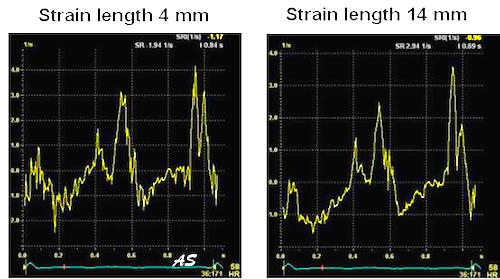
Curvature
dependency
of 2D strain
The longitudinal values that are obtained by
the 2D strain application are curvature
dependent, as shown below:
 Curvature
dependency of strain measurement. If the ROI is
curved, the midwall line will move inwards,
and thus shorten, even if there is no
shortening of the segment. This will result
in an apparent shortening of the segment
itself, adding to the real longitudinal
shortening. This curvature effect is
dependent on the curvature, the width and
the widening of the ROI.
Curvature
dependency of strain measurement. If the ROI is
curved, the midwall line will move inwards,
and thus shorten, even if there is no
shortening of the segment. This will result
in an apparent shortening of the segment
itself, adding to the real longitudinal
shortening. This curvature effect is
dependent on the curvature, the width and
the widening of the ROI.
 |
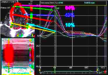
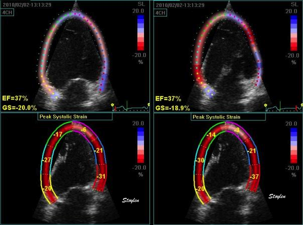
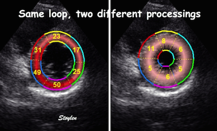
Curvature
dependency of strain in 2D strain by
speckle tracking. The two
images are processed from the same
loop, to the right, care was taken to
straighten out the ROI before
processing, while the left was using
the default ROI. In both analyses the
application accepted all segments. It
can be seen that the apical strain
values are far higher in the right
than in the left image (27 and 21% vs
19 and 17%). However, the
curvature of the ROI even affects the
global
strain, as also discussed above
in the basic
section.
|
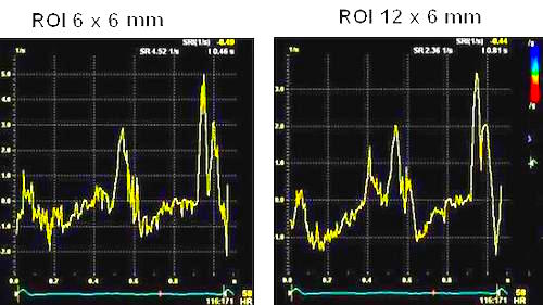
The width and thickness as well as curvature of
the ROI is non standard, defined ad hoc. In
addition, the ROI width is uniform from base to
apex, while the myocardium is thinner in the apex,
giving a discrepancy between ROI width and wall
thickness. As the curvature effect is also a
function of ROI width, this may add to the
curvature effect. This effect may account for the
observed base-to-apex gradient of strain values
observed in some studies. The combined method (and
indeed tracking of segment length by speckle
tracing alone without TDI by the same application)
is curvature independent as shown
below.
It may be the reason why some authors find a
base-to-apex gradient in the strain values
obtained by this application, while we did not in
the
HUNT study.
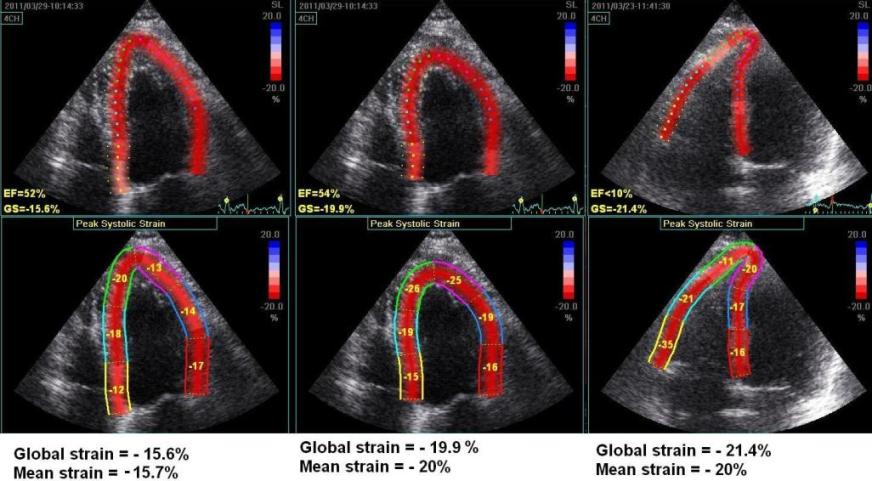 Another
instance of the curvature dependency of
measured values. The left image is processed
with fairly straight ROI in the apex. The
middle image is the same loop processed with
more curved ROI, in both cases the
application suggested acceptance of the
tracking in all segments. AS opposed
to the above example, in this case the
global strain is severely affected by the
ROI shape as well (.15.7% vs - 20%). To the
right is shown another loop from the same
patient, centered on the right ventricle. In
this case, the values of the septum is quite
similar to the values in the left image, but
differs from the middle image. The
interesting thing is that the global strain
itself is different from the mean strain
calculated from the segmental values.
Another
instance of the curvature dependency of
measured values. The left image is processed
with fairly straight ROI in the apex. The
middle image is the same loop processed with
more curved ROI, in both cases the
application suggested acceptance of the
tracking in all segments. AS opposed
to the above example, in this case the
global strain is severely affected by the
ROI shape as well (.15.7% vs - 20%). To the
right is shown another loop from the same
patient, centered on the right ventricle. In
this case, the values of the septum is quite
similar to the values in the left image, but
differs from the middle image. The
interesting thing is that the global strain
itself is different from the mean strain
calculated from the segmental values.
This may affect the
regional strain as well, as the curvature
dependency may assign higher values to
akinetic segments as shown below:

|
|
Small
apical infarct. Admitted with a
history of pain, but free of pain
and with normal ECG, but
elevated Troponin
(analysis results not ready till he
had new pain) at the time of
admittance. This Echo at
admittance was initially considered
normal, even though by retrospective
evaluation there is a small area of
hypokinesia with delayed
onset in the apex.
He then had recurrent pain after a
few hours, with ST-elevation.
|
The
colour M-mode clearly shows the
delayed onset (Apical part
starting blue), and the time delay
can be measured. Also. the colour
is lighter, and more seckled,
showing qualitatively thet the
contraction is reduced. |
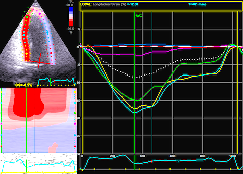
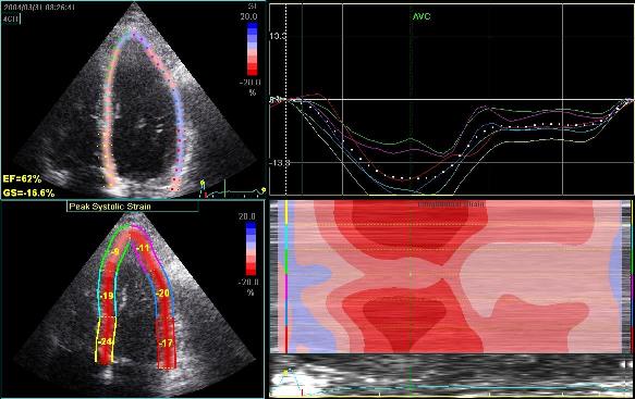
Tissue Doppler based strain rate
and strain showing hypokinesia in the
apex (yellow and red curves) , peak
systolic strain of - 5% and -8%, strain
rate of - 0.35 and -0.8 s-1
both segments with post systolic
shortening, as contrasted with normal
deformation in the base (green and
cyan). This is an indication of a small
ischemic insult at the time of the first
pain episode as also shown by the
troponin results.
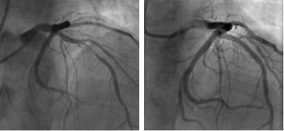
Angiography
at the time of recurrent pain showed a
tight LAD stenosis (top), confirming the
strain findings, it was treated with PCI
and stent (bottom) in the same
procedure. Strain and strain rate values
were normal after one week.
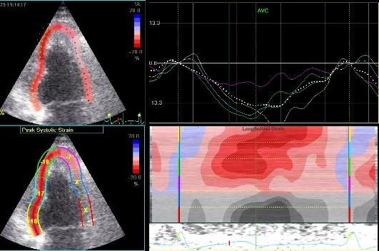
 2D
strain of the same recording (B-mode
loops without TDI). The curved M-mode
gives apical strain of -14
and -15%, i.e. borderline normal.
This was the default ROI.
2D
strain of the same recording (B-mode
loops without TDI). The curved M-mode
gives apical strain of -14
and -15%, i.e. borderline normal.
This was the default ROI.
 Adjusting
the ROI making the apical segments
straighter, reduces apical strain to -9
and -11% (borderline abnormal)
Adjusting
the ROI making the apical segments
straighter, reduces apical strain to -9
and -11% (borderline abnormal)
Both images
were made with default (medium) spatial
smoothing, but the values did not change
more than 1% by reducing smoothing to
minimum. In this case, the curvature
effect is probably more important than
the smoothing,
although both factors may contribute.
|
|
Inferior
infarct in a rather foreshortened
view, resulting in a spherical
image. By visual assessment this
infarct is akinetic in the basal
segment
|
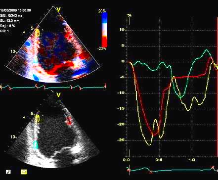
Strain
by tissue Doppler, showing
systolic akinesia in the basal
segment (cyan curve) - mark how
the ROI is placed to avoid the
lower part of the segment where
there is angle discrepancy), and
normal strain in the apical
segment (yellow) and the anterior
wall (red).
|
 |
| Strain by
2D strain, showing borderline
reduced, but still viable strain of
- 12% in the basal segment. IN this
case, the near akinetic segment has
a strain that mainly is due to the
inward motion as described in the
diagram above.
In addition, the ROI, being the same
all the way around, overestimated
the wall thickness in the infarct,
also contributing to the curvature
dependent strain, which is dependent
on the ROI width. In this case, the
effect is due to the curvature, not
smoothing,
reducing smoothing did not reduce
strain in the infarct zone at all. |
.
 Inferior
infarct. Hypokinesia of the basal segment. Not
immediately evident.
Inferior
infarct. Hypokinesia of the basal segment. Not
immediately evident.
|
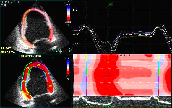
Strain and
strain rate. Basal hypokinesia and
post systolic shortening (yellow).
Also normal curves in the inferior
apex as well as in the anterior wall
(red and cyan).
|
|
|
Same
infarct as above. Tracking shows poor
tracking in the basal and midwall
segments have poor thickening due to
poor tracking. The anterior wall is
less visible. The segments are not
approved for analysis.
|
Longitudinal
strain. The apical anteior segment
shows reduced strain, but this is due
to poor tracking. The basal segment
does not show reduced systoloic
strain. However, looking at the curve,
the infarcted segment does show post
systolic shortening, so the infarct is
still indicated.
|
Transmural
and circumferential strain.
As speckle tracking is
partially angle independent, it may be applied to
the short axis as well.
However, the diverging ultrasound lines will lead
to increasingly wider speckles due to
decreasing lateral resolution as discussed
above.
In short axis images, this might lead to problems,
esopecially with circumferential strain in the
inferior segments:
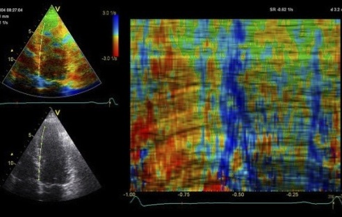
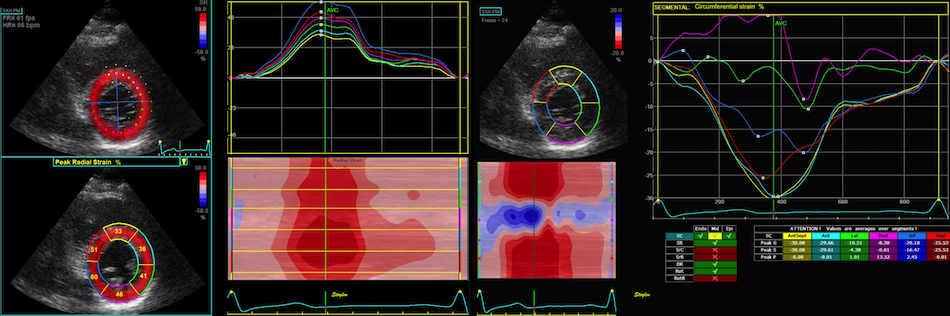 Image from a healthy subject.
Transmural strain seems fair, in the septum
and inferior wall tracking is along the
ultrasound beam, with good axial
resolution. But even tracking
laterally in the septum and lateral wall,
the curves and values make sense. In the
inferior wall, however, the lateral
resolution is so poor, that the curves are
abnormal due to ttracking artefacts.
Image from a healthy subject.
Transmural strain seems fair, in the septum
and inferior wall tracking is along the
ultrasound beam, with good axial
resolution. But even tracking
laterally in the septum and lateral wall,
the curves and values make sense. In the
inferior wall, however, the lateral
resolution is so poor, that the curves are
abnormal due to ttracking artefacts.
However, as there is between 1 to1.5 cm out
of plane motion of the base, and about half that
in the midwall, the imaging plane contains
different parts of the LV in systole and diastole,
speckle tracking in short axis views actually
don't see the same acoustic markers in systole and
diastole, so it's not real speckle tracing in the
sense that the same speckles are tracked
throughout the heart cycle, as discussed
above.
This also means that
the speckles that are tracked do not
represent physical myocardial points.
Thus, the physiological meaning of transmural and
circumferential strain becomes slightly dubious.
However, this do not only pertain to 2D strain.
This remains a caveat when new measures are added.
In the question of rotation, especially torsion,
the spiral course of the longitudinal fibres may
even cause the displacement to cause the fibres to
be traced as rotating around the cavity centre.
The speckles may
be the endocardial borders, or even the fibres
that may run in spiral. Thus, in the base, the
physiological meaning of the obtained values is
questionable.
Accepting the validity of speckle tracking in
short axis views, it then allows tracing of
transmural and circumferential strain. Transmural
strain is wall thickening, and the tracking in the
transmural direction will be dependent on the
resolution, which is better along the ultrasound
beam than laterally. The physiological meaning of
circumferential strain, shouold be midwall
circumferential shortening, which actually is
nothing more than

* midwall fractional
shortening as reasoned
above.

|
|
|
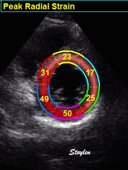
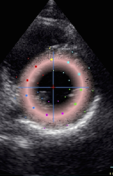
2D strain
applied to short axis image. Again
this can be seen to track in two
dimensions, the thickness following
the wall thickening, and the mid line
in the ROI Showing midwall
circumferential shortening.
|
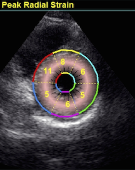
Transmural
strain. In this image the application
only measures between 10 and 15%
transmural strain, while the true
values in a normal person as this may
be as high as 40 - 50%. This is
probaly due mainly to a too thick ROI
(default), although poor lateral
tracking combined with smoothing
may contribute.
|
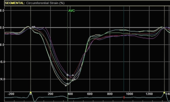
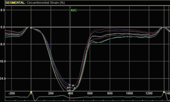
Circumferential
strain from the same
processing. In this image
about 15%, which is closer to normal.
This, however, does not mean that the
circumferential strain is more
reliable, it means that the thickness
error in the ROI is compensated by an
underestimation of the cavity volume.
It's equivalent to the fractional
shortening increasing in
hypertrophy, despite reduced wall
thickening. (Actally
circumferential strain = * midwall FS. )
|
Width of the ROI
Transmural strain all thickness and wall
thickening. But in the 2D strain application, this
means ROI width as shown below.
|
|
Normal ventricle in short axis
view.
|
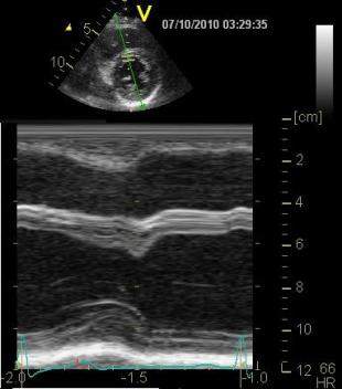
The loop
can be used to generate an anatomical
M-mode, the line is skewed to avoid
the papillary muscles. On this M-mode
the following values were measured:
LVIDD: 53mm ,LVIDS: 36mm, giving a FS
of 32%, IVDS 7 mm, IVSS 11mm, giving a
wall thickening of 57%, LVPWD 8mm,
LVPWS 11mm, giving a wall thickening
of 38%, and a mean wall thickening of
48%.
|
Below are shown transmural strain by 2D strain
with different ROI width. The images are all
processed from the loop above, and endocardium
traced in standard manner. In reprocessing, only
ROI width was changed without changing the initial
contour. All ROI's were accepted by the analysis
software for all segments:
 |
|
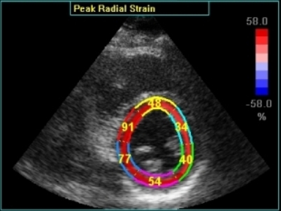
Transmural strain with narrow
ROI setting. Tracking seems
fair. In the septum, tracking is
good, but the relative wall thickening
is absurd, 77 and 91!; normal
endocardial motion in absolute terms,
gives a too high relative wall
thickening in percent of the narrow
ROI. Thanks to Ben Bulten of the
Univerity of Twente, who pointed out
that the image in this frame was
erroneous.
|
 |
|
Transmural
strain with default (medium) ROI
setting. Tracking
seems fair.
|
 |
|
Transmural strain with a wide
ROI setting. Tracking
seems fair. Mean WT =
37%, because a normal endocardial
motion in absolute terms will result
in a low percentage of the too wide
ROI.
The
measured wall thickening is evidently
as expected a function of diastolic
ROI width, as expected. Compare also
mean and the relevant segments with
the values above
|
It is evident that the transmural strain is
extremely sensitive to the ROI width. This is
pertinent to long axis analysis also, as the
curvature
in
the apical segments will lead to an
increased susceptibility of the ROI width. This
may be some of the reason why Becker et al (
212)
found transmural strain even in segments with
total transmurality of scars, and not tethering as
presumed.
 |
 |
|
|
|
|
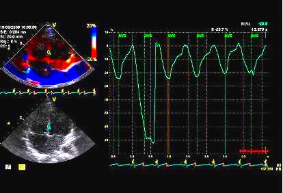
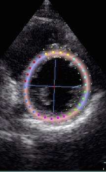
Cross section
from the same loop, processed with
a narrow (top) and wide
(bottom ROI)
|
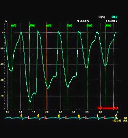
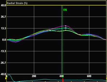
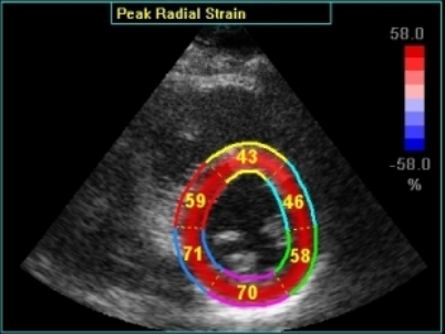
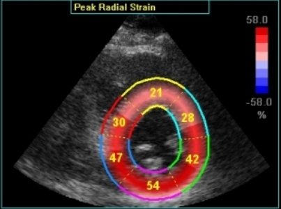
Radial strain
values from the two different ROI's to
the left, showing again a huge effect
of ROI width on transmural strain
values.
|
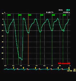
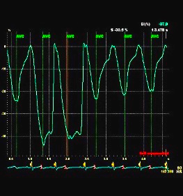
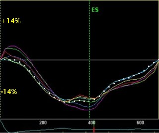
Circumferential
strain from the
same processings, the narrow sector
gives a mean circumferential strain of
-24.2%,
the wide sector -29.2. Thus, the
circumferential strain is more
dependent on the depth of the
measurement, than the width of the
ROI.
|
Repeatability
of 2D strain.
Basically, the 2D strain application, due to a
high amount of
smoothing,
should have a high repeatability, as shown
here. However, this will only be
the case as long as the tracing is done in the
same manner each time, in the same loops. This
means a very standardised endocardial tracing, and
a standardised ROI width. As shown above, the
values are extrmely dependent on the ROI, both
curvature
and
width of the ROI.
Utilising the automated features of the
application will ensure this, but will not
necessarily ensure the correct shape and
width of the ROI, and hence, not necessarily the
correct values either. In a study (
208)
where repeated measurements in the same loops was
compared for different centres, the 95% limits of
agreement were -11.4% to +11.8%, but with very
little bias. Repeated recordings within one hour
(presumably by the same observer), had limits of
agreement of -9.6 to + 9.7%.
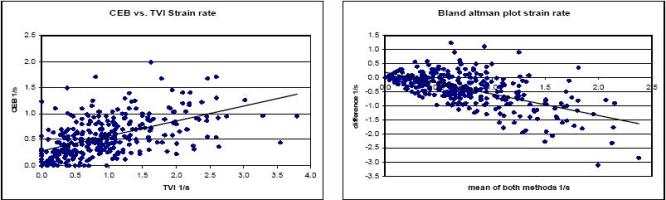
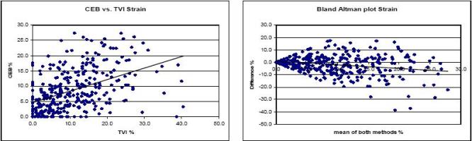
Both segmental strain and 2D strain have been
compared for longitudinal strain, and compared to
tissue Doppler (
151,
153)
as shown in
this table.
Both seem to agree fairly well. In addition
variability of strain rate (but not strain) is
lower by both methods than by tissue Doppler.
However, both Segmental strain and 2D strain use
automatic segmentation, this may be some of the
reason for better repeatability, not speckle
tracking vs. tissue Doppler per se. However, the
higher variability of strain rate by velocity
gradient, shows this method to have a somewhat
higher noise componenet. Feasibility of both
methods is reported to be between 70 and 80% of
segments (lower in the HUNT study,but this is due
to the aim of the study, to provide normal values
as free as possible from artefacts.
Summary
of differences and limitations of segmental
speckle tracking and 2D strain.
It is important to be aware of the limitations of
each method. It should also be emphasized that
different methods are not necessarily directly
comparable, and may yield different normal values
and cut offs, due to the different ways parameters
are measured. One of the fundamental differences
stem from the different geometrical assumptions
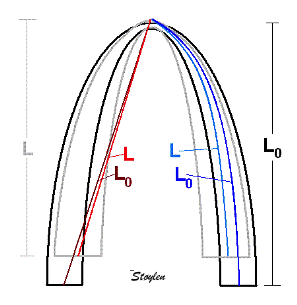
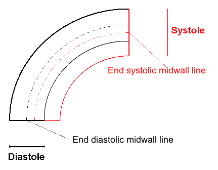
that are present as shown below:
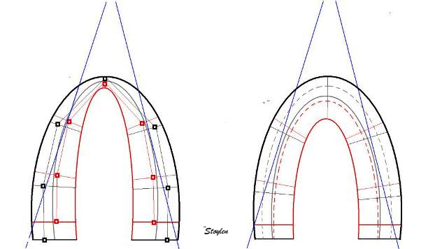
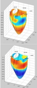
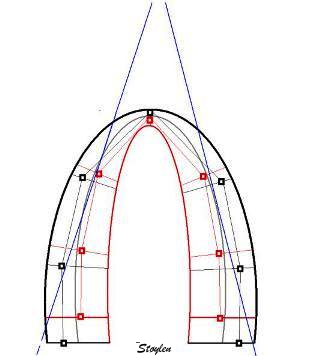
Differences in geometry between methods.
The fairly invariable outer LV contour is
shown in heavy black. The diastolic inner
contour, segmental borders, kernel
positions and measurement lines are shown
in light black. Systolic inner contour, segmental
borders, kernel positions and measurement
lines are shown in red. Left: Segmental
strain by tracking of kernels at segmental
borders. It can be seen that the main
deformation is measured along the
longitudinal axis of each segment. As the
wall thickens, the longitudinal mid line
of the segments moves inwards, but in the
basal and mid wall segments this does not
add to the shortening as the angle does
not change much. In the apex,
however, the angle of the center
line changes, contributing to the
segmental shortening when it is measured
by this method, however, the effect is
slight. To the right is shown the
geometric assumptions of the 2D strain
method. The ROI uses an assumption
of equal thickness from base to apex, and
the mid line moves with the thickening of
the contour. The segment length is
measured along the curved line, and both
the curvature and the angle contributes to
the shortening of the segment mid line as
it moves inward. Thus, the shortening
(strain) might be expected to be
higher in the apical segments by this
method, as well as being dependent on the
curvature, especially in the apex.
(However, this effect may be masked by the
high degree of smoothing inherent in the
application, which may distribute the
differences between segments.
Ultrasound beams are shown in blue,
illustrating the alignment problem of this
method, thus resulting in lower
values in segments that are poorly
aligned.
Inter
vendor differences in speckle tracking
As speckle tracking have been attempted to be a
solution to the shortcomings of tissue Doppler,
and as this can be done in ordinary B-mode. most
vendors have in time come up with speckle tracking
applications in their analysis software. Also,
vendor independent software, using the DICOM
standard, are available.
This has been an interesting development, as the
later studies have sbhown a fair amount of
variability between strain measurements by
different vendors (
373
- 382). Normal values are not sufficiently
harmonised that measures are interchangeable. For
longitudinal 2D strain, biases of 1% absolute (
373
- but here both methods had a much larger bias
against MR tagging), to 5% (
375).
and with correlations between measurements in
same-day measures in the same patients vendor
specific software as low as 0.35 (
374)
to 0.23 (
377),
but with no or less differences between different
acquisitions when analysed in the same software (
374),
suggesting that the differences in software is the
main source of variability between systems.
However,
even different versions of the same
software has been shown to result in different
measurement values (377).
In general, variability have been found to be
between 2 and 5% between software (
378).
It has been suggested that reproducibility is
better than for EF measurements, but taking into
account that EF by biplane tracings is
the
poorest reproducible parameter, this argument does
not impress much.
Reproducibility within the frame of one software
vendor, is much better, not surprising as
discussed years ago in the paragraph
above,
the
smoothing
will always yield good repeatability (in fact, if
you smooth the curves to zero, repeatability will
be 100%), but still it has been found to be
unacceptably high in newer studies, even within
the frame of one software (
377).
Although some researchers have found a fair
correspondence between global strain measurements,
(
376),
reproducibility of regional strain is much
poorer. Reproducibility is not better in 3D
speckle tracking (
379-383).
Also, the 3D camp maintains that automated 3D
volume and EF is far more reproducible, and thus
the balance may tip away from 3D strain.
The variability is not especially
surprising!
As discussed years ago, how the strain is defined
has an impact on measurements especially the
length of the wall.
Curvature
dependency of the ROI is also an issue, in a
wide ROI, the inward motion (which is really
circumferential shortening) will be interpreted as
longitudinal strain. And this again is dependent
how wide the ROI is defined in the apex.
This of course, not only affects the performance
of different softwares, but also the
repeatability, which in newer studies are much
lower than previously reported (
377),
not surprising seeing the randomness of basic
settings in ROI size and shape.
Of course, the number of speckles included in
analysis, the definition of stability of speckles
as this will define the amount of
drift
that is permitted by the software, and these are
also specific to each. Finally, the amount and
type of smoothing may vary.
The main limitation of any echo method is the
ones related to data quality.
AS discussed under each method;
- The fundamental limitations related to all
methods are the ones arising from:
- Tissue Doppler, having the advantage of high
frame rate has additional limitations related
to:
- Speckle tracking (in any form), being less
angle dependent has additional limitations
relating to:
- Segmental strain, being robust and giving
the opportunity of utilising both
tissue Doppler and speckle tracking and
eliminating the angle problem, has the
additional problem of:
- The 2D strain application, being robust and
user friendly, has the additional problems of:
- Smoothing,
relying heavily on AV-plane motion,
- which may give strain values even where
there are none, and may reduce sensitivity
for reduced regional function
- Makes the tracking more difficult to
assess visually
- Curvature
dependency, due to the technicalities
of the specific applications, which may give
too high values in the apex.
- ROI
width seems to be critical, espacially
in transmural strain.
How do the methods compare?
Going through a challenging case:

|

|
There is
hypokinesia in the apicoseptal
segment. The lateral wall seems to
move fairly OK, almost to the apex. In
addition, there is nearfield clutter,
more pronounced in the lateral part,
and a stationary reverberation in the
lateral base.
|
Looking at peak
values from the speckle tracking
application in a bull's eye pliot,
there is -18% strain in the
apicoseptal segment, as well as -22%
in the basal lateral. However, there
is apparent hypokinesia in the apical
and mid lateral wall.
|
However, as curve shapes generally gives more
information, curves are given here:
 There is an apparent hyperkinesia in
the basal lateral wall, which is due to the
segment being "squeezed" bwetween the mitral
ring and the lateral wall. There are lower
strains in the region of nearfield clutter,
but also due to the reverberation, taking
away the motion of the basal border of the
mid segment. However the hypokinesia seems
to have been smoothed away. This smoothing
may also be influenced by the clutter
regions.
There is an apparent hyperkinesia in
the basal lateral wall, which is due to the
segment being "squeezed" bwetween the mitral
ring and the lateral wall. There are lower
strains in the region of nearfield clutter,
but also due to the reverberation, taking
away the motion of the basal border of the
mid segment. However the hypokinesia seems
to have been smoothed away. This smoothing
may also be influenced by the clutter
regions.
 Comparing with tissue Doppler derived
curves, the pathological apicoseptal segment
is clearly visible, both by curve shape, and
values. The tissue Doppler is even more
vulnerable to clutter, but as every ROI is
processed separately, there is no carry over
effect to segments with good image quality.
Comparing with tissue Doppler derived
curves, the pathological apicoseptal segment
is clearly visible, both by curve shape, and
values. The tissue Doppler is even more
vulnerable to clutter, but as every ROI is
processed separately, there is no carry over
effect to segments with good image quality.
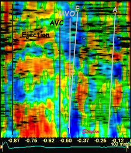
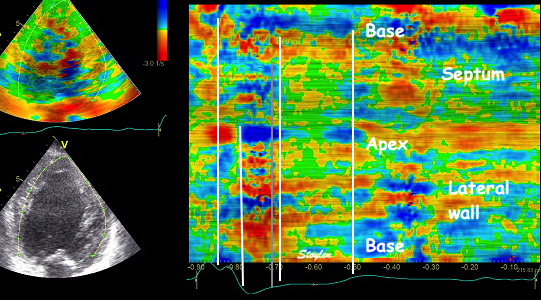
 The same patholgy is visible in the
apicoseptum by the time course in this
M-mode, but it also serves to show how badly
affected TDI is by the clutter in the
lateral wall. However, timing of the main
phases (Ejection, E, A, is still visible.
The same patholgy is visible in the
apicoseptum by the time course in this
M-mode, but it also serves to show how badly
affected TDI is by the clutter in the
lateral wall. However, timing of the main
phases (Ejection, E, A, is still visible.
In large infarcts, they seem to give about the
same information:
 |
 |
Pathology is evident, both
in M-mode
|
And in strain / strain rate
|
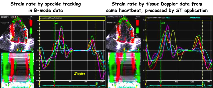
 Strain rate curved M-modes from tissue
Doppler (left) and Speckle tracking (right).
The speckle tracking image is much more
smoothed, in time due to lower frame rate of
B-mode compared to tissue Doppler. IN depth
due to the
spline smoothing of the 2D strain
application. However, in this case, the
resolution is sufficient to show intial
stretch, apical hypokinesia and post
systolic shortening also by 2D strain.
Strain rate curved M-modes from tissue
Doppler (left) and Speckle tracking (right).
The speckle tracking image is much more
smoothed, in time due to lower frame rate of
B-mode compared to tissue Doppler. IN depth
due to the
spline smoothing of the 2D strain
application. However, in this case, the
resolution is sufficient to show intial
stretch, apical hypokinesia and post
systolic shortening also by 2D strain.
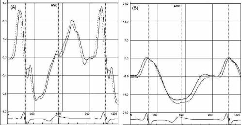
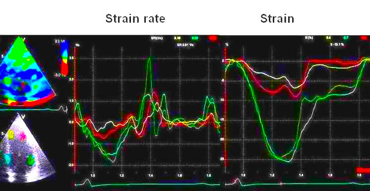
 This can also be seen in strain rate
curves, the magenta curve in the left panel
and the cyan curve in the right panel are
from the middle septal segment. The
scales on the TVI and speckle tracking are
not equal.
This can also be seen in strain rate
curves, the magenta curve in the left panel
and the cyan curve in the right panel are
from the middle septal segment. The
scales on the TVI and speckle tracking are
not equal.
 And in this case, the strain values do
show the infarct, both as curves, peak
values and on the bull's eye map.
And in this case, the strain values do
show the infarct, both as curves, peak
values and on the bull's eye map.
In this case, the infarct was rather large, and no
method had any trouble in diagnosing it (nor has
B-mode).
The next case is a small apical infarct:
 Again, the SRI CAMM from speckle
tracking has much less resolution both in
time (due to lower frame rate) and space
(due to smoothing).
The apical hypokinesia cannot
be seen, but the presence of initial stretch
as well as post systolic shortening in the
apex might be considered (but is far less
evident than in TDI). Also in this case, the
time course seems to give most information.
Again, the SRI CAMM from speckle
tracking has much less resolution both in
time (due to lower frame rate) and space
(due to smoothing).
The apical hypokinesia cannot
be seen, but the presence of initial stretch
as well as post systolic shortening in the
apex might be considered (but is far less
evident than in TDI). Also in this case, the
time course seems to give most information.

|
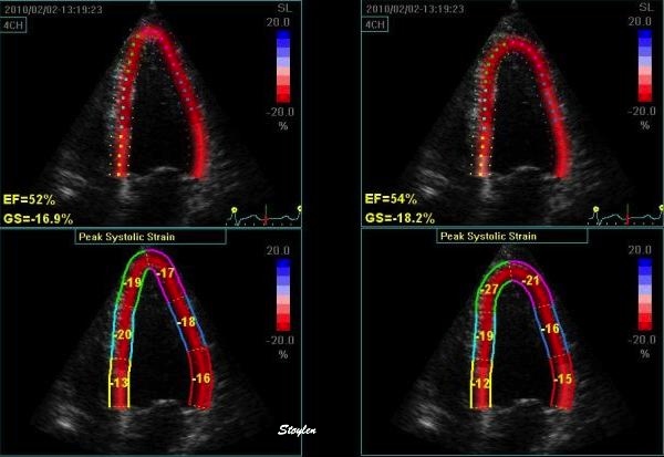
 |
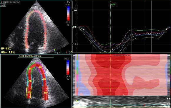
Here, the peak
systolic strain in the apex of -14 and
-15 is near normal, and the Bull's
eye of peak values is not convincing
either. There might be a slight
discernible PSS in the two apical
curves (green and cyan), but this is
also within normal range. Time course
in SR CAMM seems to be the best
indicator.
|
TDI strain shows
a peak systolic strain of -6,
and evident PSS.
|
In this case both
smoothing
and
curvature
dependency might contribute to hide the
apical dysfunction.

|

|
| In case
6, the peak strain in the
inferobasal segment is reduced, but
might be interpreted as inaccurate
processing when seen in the bull's eye
view. The best clue to the infarct
is the curve
from the basal segment (yellow)
showing reduced systolic strain and
post systolic shortening, i.e. the
time course, but in this case the
hypokinesia is evident. |
And in this case
both curves and values correspond with
the two methods
|
In this case, the inferior infarct is visible. In
another, nearly similar case, however, the infarct
was not very visible in speckle tracking:
 |

|
| Strain by tissue
Doppler, showing systolic akinesia in
the basal segment (cyan curve) - mark
how the ROI is placed to avoid the
lower part of the segment where there
is angle discrepancy), and normal
strain in the apical segment (yellow)
and the anterior wall (red).
|
Strain by 2D
strain, showing borderline reduced
strain of -12% in the basal segment.
In this case, the strain is due
to the inward motion (by tethering)
which reduces the length of the curved
segment. In addition, the ROI, being
the same all the way around,
overestimates the wall thickness in
the infarct. In this case, the effect
is due to the curvature, not
smoothing. |
Finally where there are drop outs, the spline
smoothing may distribute the motion over fewer
segments, thus masking the infarct totally:
 Stiff inferior wall due to an infarct,
but fair annulus motion due to normal, or
even hyperkinetic apical segments.
Stiff inferior wall due to an infarct,
but fair annulus motion due to normal, or
even hyperkinetic apical segments.
 - which results in the normal
annulus motion being splined over only three
segments, instead of six, as there is a
drop out of the whole anterior wall, and the
segments are excluded, as opposed to TDI where
analysis is only local.
- which results in the normal
annulus motion being splined over only three
segments, instead of six, as there is a
drop out of the whole anterior wall, and the
segments are excluded, as opposed to TDI where
analysis is only local.
Back to
main website index.
 Editor:
Asbjørn Støylen Contact address:
asbjorn.stoylen@ntnu.no
Editor:
Asbjørn Støylen Contact address:
asbjorn.stoylen@ntnu.no