The main principle of B.mode measurement is to assess wall thickening in moving images. It can be done iether semi-quantitatively in wall motion score. Wall thickening can also be measured quantitatively as transmural strain.
 |
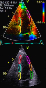
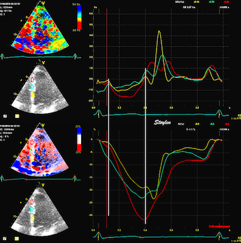
| Velocity imaging. Velocities toward the probe is coded red, away from the probe is blue. Thus the ventricle is red in systole, when all parts of the heart muscle moves toward the probe (apex) and blue in diastole, but the colours are representations of actual numerical values.. |
 |
 |
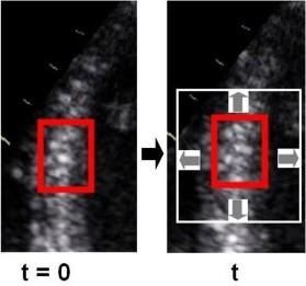 |
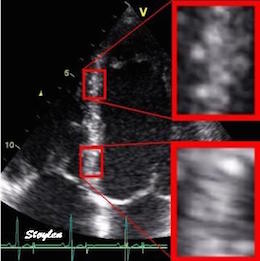
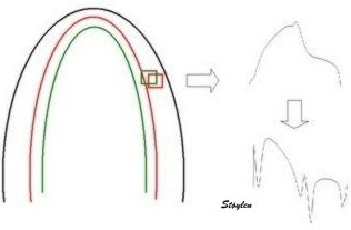
| The two enlarged areas show completely different speckle patterns. | As the speckle pattern in addition
is relatively stable; |
This can be used for a search for the best matching kernel in the next frame, within a specified search area. |
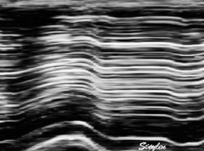
| The angle error in displacement measurement demonstrated in a reconstructed M-mode. As the skewed M-mode line is shorter, scales have been lignes at 0 and 6 cm (green lines). But the caliper measures are showing how increasing angle between M-mode line and direction of motion increases the overestimation of the MAPSE. | Measuring mAPSE by an
M-mode along the ultrasound beam, may give an angle
deviation compared to the motion of the mitral ring, but
as seen this angle deviation is small. |
 |
|
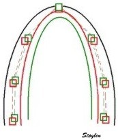
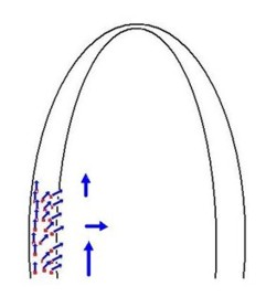
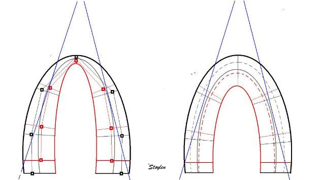
| Curvature dependency of
strain measurement. If
the ROI is curved, the midwall line will move inwards,
and thus shorten, even if there is no shortening of the
segment. This will result in an apparent shortening of
the segment itself, adding to the real longitudinal
shortening. This curvature effect is dependent on the
curvature, the width and the widening of the ROI. |
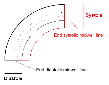
Effect of a curved ROI on
strain. As the ventricle shortens, the wall thickens,
which means the wall thickens. Systolic outer (red),
midwall (yellow) and inner (blue) lines are shown in the
diastolic frame to the left. In the systolic frame to
the right, the same lines are shown in diastole, while
the corresponding systolic lines are shown as dotted,
thin lines to illustrate the motion. There is little change of the outer ROI contour, while the midwall line moves more inward, due to thickening of the outer half of the wall. This will add to the shortening of the midwall line, due to the effect described to the left. Mean longitudinal strain will be closest to the midwall line shortening. The endocardial line will move even more inwards, by the thickening of the whole wall, and thus have even more curvature dependent shortening. |
As seen by the example above, in speckle tracking derived strain, the curved ROI will result in an additional shortening due to the inward motion of the curved lines. Thus, speckle tracking strain is expected to show higher absolute values for GLS. A large meta analysis gave mean normal values of 19.7% (427), but the study was unable to show age or gender variability due to large inter study heterogeneity. The NORRE study (457) found in a single center speckle tracking study a GLS of mean 22.5 % (SD2.7). This is as expected.
However, there are additional assumptions that will differ between
vendors of speckle tracking programs. Using mean strain over the
ROI will result in a value close to the mid ROI line. Some
vendors, however, trace the endocardial line, which will result in
higher absolute values. The thickness of the ROI is often assumed
to be constant, while the wall is thinner in the apex. As the apex
is the most curved part, a ROI in the apex that is thicker than
the wall, will result in a higher absolute GLS. The curvature in
the apex may also vary, even in the same software, as shown here.

Curvature dependency of strain in 2D strain by speckle tracking. The two images are processed from the same loop, to the right, care was taken to straighten out the ROI before processing, while the left was using the default ROI. In both analyses the application accepted all segments. It can be seen that the apical strain values are far higher in the right than in the left image (27 and 21% vs 19 and 17%). However, the curvature of the ROI even affects the global strain, as also discussed above in the basic section.
Finally smoothing,
software algorithms, such as choice of kernel sizes, selection and
weighting of acoustic markers, stability of speckles, and drift
compensation during heart cycle are all assumptions that are
guarded as industrial secrets.
Thus, it is not surprising that there are inter
vendor differences, even in speckle tracking derived strain.

 |
 |
| Inferior infarct.
The basal segment is dyskinetic,
but there is a longitudinal
motion due to tehthering |
Reconstructed short
axis slices from the same patient. The slices tracks the
longitudinal motion, as seen to the left, but there is
evident dys- to akinesia in the inferoseptum in the
basal slices. |
 |
 |
 |
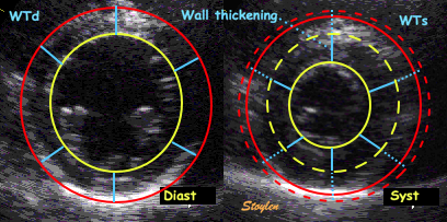
| Wall thickening. Systolic wall
thickening equals systolic transmural strain: WT = (WS
- WD)/WD = |
Wall thickening, illustrated from
the loop shown to the left. The outer (red) and
endocardial (yellow) contours and wall thicknesses are
shown in the diastolic image to the left, and
transferred to the systolic image on the right, shown as
dotted lines of the sane colour. The systolic contours
are shown as solid lines. The systolic wall thickness is
then (more or less) the dotted plus the solid blue
lines, and the wall thickening the solid blue lines. |
The transmural strain can be
measured in M-mode from systolic and diastolic wall
thickness, which will give wall thickening in only two
segments, but may be taken as representative as the mean
wall thickening in this plane where there is no
segmental dysfunction. |
It could in principle also be measured in long axis, but this is
less feasible as the basal parts of the long axis views suffer
from poor lateral resolution due to the divergence
of the ultrasound lines with increasing depth in the sector.
 |
 |
|
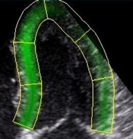
| Four chamber view with tissue
Doppler strain rate, where both ROI and strain length is
adjusted to cover about one segment. The curves obtained
by this are representative of each segment. |
Segmental strain obtained by tracking kernels at the segmental borders, calculating the distance in each frame, deriving the Lagrangian strain for each segment. | Automated segmentation by a speckle
tracking method. In this application there is speckle
tracking, but the results are partly smoothed along the
whole ROI (all six segments) by a spline function. The
segmental values then obtained are the average of the
spline function for each segment. |
 |
 |
 |
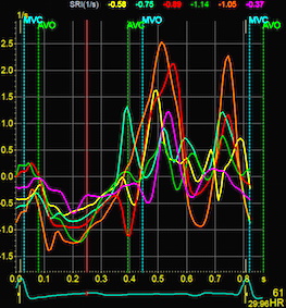
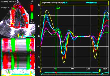
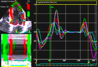
| Strain rate curves from the
recording above, each curve is representative of a
segment. |
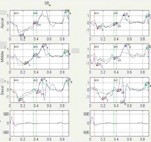
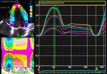
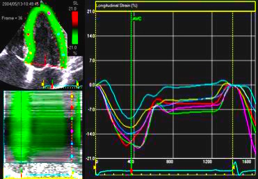
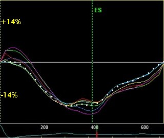
Segmental strain rate curves from the application above, obtained by temporal derivation of the Lagrangian strain and converting to Eulerian strain rate. | Strain curves abd peak systolic
values from the recording above. Each curve and value
are representative for the spline function in each
segment. (In this image, there is little evidence for
any strain gradient from base to apex!) |
 |
 |
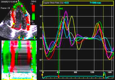
| Strain rate is calculated as the velocity gradient between two spatial points, the pixel strain rate value being the mid point SR value. | And thus pixel strain rate values can be mapped: Strain rate is coded yellow to orange for shortening, cyan for lengthening but green in periods of no deformation, but the colours are representations of actual numerical values. |
|
 |
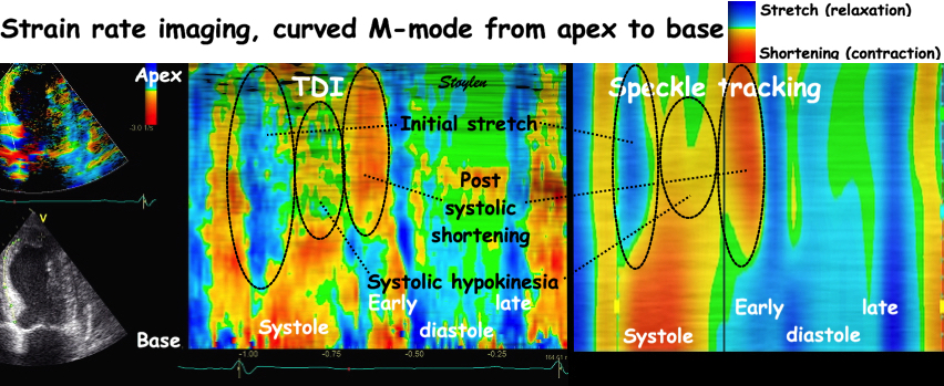
| Combined strain rate image with one systolic and one diastolic frame displaued in B.mode, below, the CAMM from the septum and below that, the strain rate (yellow) and strain curves from one point in septum. |
| V-plot of the
velocities from a four chamber view. The slope of the
v-plot is the strain rate. |
Strain rate and strain can be visually assessed by the offset
between the curves, when the velocity curves are obtained from
points with a known (and equal) distance.
The velocity gradients van be mapped onto the representation of a wall. This is a semi quantitative plot of the values, but it will give quantitative timing information.
The parametric
display of curved M-mode is most useful in strain rate,
showing the quick shifts in negative and positive strain rate. It
enables:
 |
 |
 |
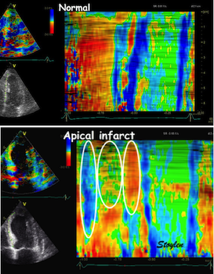
| Colour M-mode can show the presence
of disturbed regional function (as here by the initial
stretch, reduced contraction and post systolic
shortening in the apical segment in the infarct in the
bottom panel). It can even show changes with better
spatial resolution, showing sub segmental extent
of changes. |
Colour M-mode can be used semi-quantitatively for wall motion score, although this is longitudinal strain, not wall thickening, this has been shown to be equivalent (6, 7). | Curved M-mode can also be used
quantitatively for timing information. The timing
differences between different parts of the myocardium,
is important additional information, and can be seen to
be fairly robust despite the presence of heavy clutter
noise in this image. |
 |
 |
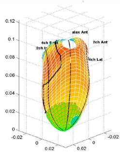
| Strain rate 3D mapping in time. The problem with the moving loop is the same as in 2D display. During ejection there is a short period with homogenous colour, when all the ventricle shortens simultaneopusly. But during diastole, there is a continuously shofting array of colours, as different parts of the ventricle elongates at different times. the continuously shifting colours are not easy to interpret. In addition it won't show all of the surface simultaneously. (Image courtesy of E. Sagberg.) | Strain rate 3D mapping in space. Stopping the frame in one point in systole shows a fairly even distribution of colur (yellow - shortening), meaning an image with normal systolic function and fairly free from artefacts. In order to see all of the surface, however, the image has to be rotated.(Image courtesy of E. Sagberg.) |
 |
 |
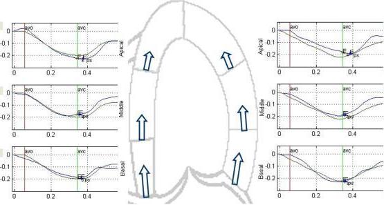
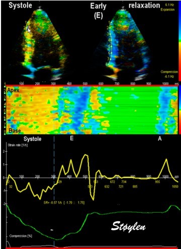
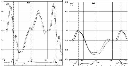
| Normal subject. Strain rate (top)
shows the changes in deformation, while strain (bottom)
shows the deformation statur at any given point in time.
Thus, quick changes will only show up in strain curves
as changes in the direction of the curves. This is
especially evident when looking at the diastole. |
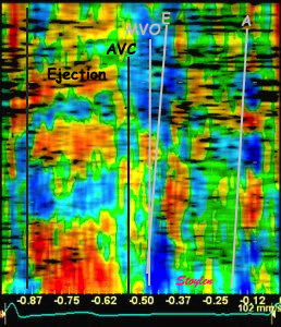
In this case with a large antero
apical infarct, changes in
segmental deformation from stretch to shortening during
ejection is evident with strain rate (top), but not in
the strain curves (bottom). Peak rate of change in
any phase can be measured by strain rate, not by strain.
Changes in strain (i.e. strain rate) can be
puzzled out qualitatively, if one looks at the
changes in direction of the curves (which in fact is
strain rate). The main impression from strain,
however, is the systolic stretch in the two apical
segments. |
 |
 |
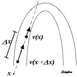
| Kernel displacement. Following the kernel through a whole heart cycle, will lead to a displacement curve shown to the right. Temporal derivation (displacement per time, or frame by frame displacement divided by the time between frames) results in the derived velocity curve shown below. | From
two different kernels, the relative displacement and
hence, strain as well as strain rate can be derived. The
strain obtained by simply subtracting the two
displacements and dividing by the end diastolic distance
is the Lagrangian
strain. To obtain the Eulerian
strain rate, the correction has to be applied for
each frame. |
 |
 |
| If Kernels are placed at the segmental borders, the result will be segmental strain and strain rate in six segments per plane. | Placing the kernels in mid
myocardium in a short axis view, it can also be used for
trackinglobal and regional circumferential
strain and rotation in the imaged plane. |

 Longitudinal speckle tracking, with kernels at the segmental borders in four chamber view. |
 Longitudinal speckle tracking, but done crosswise in parasternal long axix view. |
 |
|
 |
| Combined search by tissue Doppler and speckle tracking. The kernels are shown as the small, round, yellow circles. The longitudinal search area along the ultrasound beam by tissue Doppler is shown in red. The lateral search area by speckle tracking is shown in white. | The result is tracking of
segmental borders. The strain is the relative change
in segment length, and the strain rate the strain
change per time. |
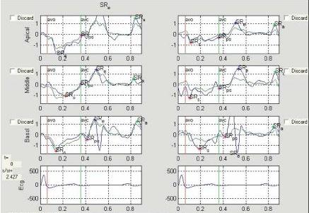
Display of segmental
strain rate from the six segments. |
 |
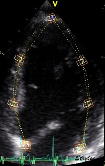
| Visualisation of the tracking. Observe how the bullets in the midline follows the myocardial motion. However, due to the smoothing function of the application, this may be virtual tracking, being extrapolated from AV-plane motion, thus the true tracking of the local tissue may be difficult to assess. |
 2-dimensional strain by
speckle tracking. Each red point represents a
kernel for speckle tracking. Velocity and displacement
decreases from base to apex, and the differential
motion along the segment gives longitudinal strain and
strain rate. As the true direction of the motion is
tracked in this instance, the transverse component can
also be tracked, and the differential motion from
kepi- to endocardium can also be tracked., giving
transmural strain and strain rate.
|
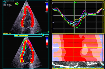
 2D strain in practice. The
midwall line is used for the longitudinal strain,
being an average of all points in the wall. The ROI
follows the wall, the limits can be seen diverging in
systole, converging i n diastole, giving the
transmural strain and strain rate at the same time.
The colours show longitudinal strain rate, green is
shortening and red is lengthening.
|
 In order to make the
speckle tracking more robust, values are averaged over
a whole segment.
|
 |
 |
| Longitudinal
velocity |
Longitudinal
displacement |
 |
 |
| Longitudinal
strain
rate |
Longitudinal
strain |
 |
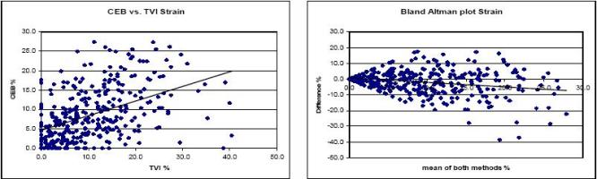 |
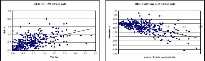
| Strain rate and strain, comparison of 2D strain and Tissue Doppler. There is a considerable spread between methods, but most probable due to variability of especially of tissue Doppler. There 2D strain gives lower values than DTI, and this tendency increases with increasing strain rate/strain. The term "CEB" meaning "computerized eye balling" was an early term to describe the application. |
|
 |
|
|
|
| Wall
thickening. Systolic wall
thickening equals systolic
transmural strain: WT = (WS
- WD)/WD =
|
Wall
thickening, illustrated from the
loop shown to the left. The
outer (red) and endocardial
(yellow) contours and wall
thicknesses are shown in the
diastolic image to the left, and
transferred to the systolic
image on the right, shown as
dotted lines of the sane colour.
The systolic contours are shown
as solid lines. The systolic
wall thickness is then (more or
less) the dotted plus the solid
blue lines, and the wall
thickening the solid blue lines.
|
The
transmural strain can be
measured in M-mode from systolic
and diastolic wall thickness,
which will give wall thickening
in only two segments, but may be
taken as representative as the
mean wall thickening in this
plane where there is no
segmental dysfunction. |
It could in principle also be measured in
long axis, but this is less feasible as
the basal parts of the long axis views
suffer from poor lateral resolution due to
the divergence
of the ultrasound lines with increasing
depth in the sector.
 |
 |
| Normal long
axis image. The motion of the
base of the ventricle towards
the apex is evident in the long
axis view. |
Lopoking at
the short axis view from the
base, this is not evident, but
comparing with the image on the
left, this mus mean that during
systole, an entirely new part of
the ventricle moves into the
imaging plane. |
 |
|
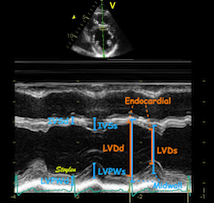
| As can be
seen, the base of the heart
moves through the M-mode line
during the heart cycle. |
This means
that measurements in fact are
taken from different part of the
ventricle in end diastolie and
end systole. It seems to
indicate that systolic
measurements are done in a part
of the ventricle with narrower
lumen and thicker wall, thus may
over estimating both fractional
shortening and wall
thickening. |
 *
midwall fractional shortening as reasoned above.
*
midwall fractional shortening as reasoned above.
 |
 |
|
| 2D
strain applied to short axis
image. Again this can be seen to
track in two dimensions, the
thickness following the wall
thickening, and the mid line in
the ROI Showing midwall
circumferential shortening. |
Transmural
strain. In this image the
application only measures
between 10 and 15% transmural
strain, while the true values in
a normal person as this may be
as high as 40 - 50%. This is
probaly due mainly to a too
thick ROI (default), although
poor lateral tracking combined
with smoothing
may contribute. |
Circumferential
strain from the same
processing. In this
image about 15%, which is closer
to normal. This, however, does
not mean that the
circumferential strain is more
reliable, it means that the
thickness error in the ROI is
compensated by an
underestimation of the cavity
volume. It's equivalent to the fractional
shortening increasing in
hypertrophy, despite reduced
wall thickening. (Actally
circumferential strain = *
midwall FS. ) |
| Method 1: segment length
by TDI and ST |
Method 2: Velocity
gradient (stationary ROI) |
Method 3: Dynamic
velocity gradient (tracked ROI) |
Method 4: 2D strain (AFI)
|
|||||
| Peak Strain rate |
End systolic Strain |
Peak Strain rate | End systolic Strain | Peak Strain rate | End systolic Strain | Peak Strain rate | End systolic Strain | |
| Apical | -1.12
(0.27) |
-18.0 (3.6) |
-1.46
(0.85) |
-14.6 (9.0) |
-1.31
(0.73) |
-17.2 (9.1) |
-1.12
(0.37) |
-18.7 (6.6) |
| Midwall |
-1.08
(0.22) |
-17.2 (3.2) |
-1.29
(0.56) |
-18.2 (7.4) |
-1.40
(0.58) |
-16.9 (7.1) |
-0.99
(0.23) |
-18.3 (4.7) |
| Basal |
-1.03
(0.24) |
-17.2 (3.5) |
-1.71
(0.94) |
-19.6 (9.3) |
-1.59
(0.74) |
-17.1 (8.6) |
-1.12
(0.36) |
-18.0 (6.2) |
| Mean |
-1.08 (0.25 |
-17.4 (3.4) |
-1.45
(0.79) |
-17.7 (8.5) |
-1.43
(0.67) |
-16.7 (8.1) |
-1.07
(0.33) |
-18.4 (5.9) |